H-Model
It is a quantitative method used in stock valuation to linearly decline the high growth of a stock towards the terminal year


What Is The H-Model?
The H-model is a modified dividend discount model (DDM), part of the Discounted Cash Flow (DCF) method.
Before we look further into this model, it is necessary to have some understanding of DDM. The dividend discount model with constant growth is also known as Gordon Growth Model (GGM).
As a valuation tool, this model assumes that a company’s stock’s value equals the sum of its future dividends. Based on the net present value of future dividends, the formula of DDM, assuming dividends grow at a constant rate, is:

In the formula, the variables are:
- P: Current stock price
- D1: Value of the dividend at the end of the first period
- r: Company’s constant cost of equity capital
- g: Constant growth rate
To understand the equation above more easily, we transform the formula into:

Where D1/P0 is the dividend yield, g is the growth rate, and r is the total cost of equity. This formula can also be represented as
Total Return = Income + Capital Gains
There are several notable shortcomings of the DDM. First, in some cases, assuming that an eternally stable growth rate will be less than the cost of capital is unreasonable.
I. If the stock does not currently pay a dividend, like many growth stocks, the stock must be evaluated using a more general discounted dividend model.
II. The stock price depends heavily on the growth rate g chosen in the Gordon Model.
Another model worth noticing is the two-stage model. Like the model, it assumes the growth rate experiences two periods.
In the first period, dividends will increase by a fixed rate in the expected time. In the second period, we still assume dividends increase, but by a different growth rate. We will talk more about the two-stage model later.
In the model, a decline in the growth rate is a gradual process, so the model makes this process linear. As a valuation tool based on DCF, the model makes the short-term growth rate’s transition to the long-term sustainable growth rate more realistic.
- The H-Model enhances stock valuation by modifying the Dividend Discount Model (DDM) to address perpetual growth assumptions.
- Primarily for stock evaluation, it considers short- and long-term growth rates, along with the time value of money.
- Involves the Gordon Growth Model (GGM) and a transitory growth phase, incorporating the concept of half-life for gradual growth rate decline.
- It differs from the two-stage model by assuming linear changes in growth rates during the initial stage, suited for companies with initially high growth rates.
- H-Model assumes linear initial growth rate changes, suitable for firms with high initial growth.
- Modeled with UPS, estimating stock value via dividends, growth rates, and required return, stressing reliable input importance like discount and growth rates.
What is the Purpose of the H-Model?
This model is used to assess and evaluate a company’s stock.
To understand the purpose better, we need to address factors that may impact a company's stock value:
1. Short- & long-term growth rate
2. The time value of money
A first-mover and/or competitive advantage can be generated when a company releases a new product or service. Hence, investors usually give value to companies with strong growth in the short term.
However, this extra value might be transient. As time goes by, the public accepts new products or services, and competitors may release similar products or services. Thus, it is difficult for investors to determine a company's potential growth in the long run.
Here, the H-model allows a transition from a high-growth period in the short term to sustainable long-term growth.
Additionally, the time value of money is one of the most important factors affecting the value of a stock. The time value of money shows that a dollar today has more value than a dollar tomorrow since we can use the money to invest and gain interest.
Depending on the situation, investors use a discount rate and a percentage of initial investment to adjust the current value of future income.
When using the discount model, analysts use the discount rate to ascertain the present value of future dividend payments and reveal the time value of money.
For example, if you want to have $10,500 in a year at an interest rate of 5%, you need to invest $10,000 today. The present value of $10,500 at a discount rate of 5% is $10,000.
Below is a video explanation of how to use the H-Model in valuation:
What is the H-Model Formula?
As a special form of a two-stage model, calculations can be divided into two parts and added together.
The first component of the model ignores the high growth rate period and considers the stock value based on the long-term growth rate. Then, in second part considers the value from the high-growth rate period.
First, we look at the calculation of this model:

Where,
- P0: Value of the stock or equity
- D0: Per-share dividend received in the present year
- g1: Growth rate in the short term/in the company’s high growth phase
- g2: Growth rate in the long term/in the company’s mature phase
- r: Rate of dividend growth in the present year
- H: Half-life of the high-growth rate period
With the concept of the calculation and all its components, we can take a deeper look at each part of the formula.
1. The Gordon Growth Model (GGM)

This model is the core of the H-model. It is a single-phase, terminal growth calculation.
It takes the previous year’s dividend increased by the long-term growth rate and then divides that by the cost of equity investors' required return minus the long-term growth rate in perpetuity.
This valuation component is the value of a share without a high growth period.
2. The Transitory Growth Phase

This part assumes that the short-term growth rate transitions to the long-term growth rate by using the half-life of the transition period. This additional part calculates the excess growth of dividends.
It shows the additional value resulting from the high-growth period.
We can show both parts in the graph below to observe how growth rates change over time.
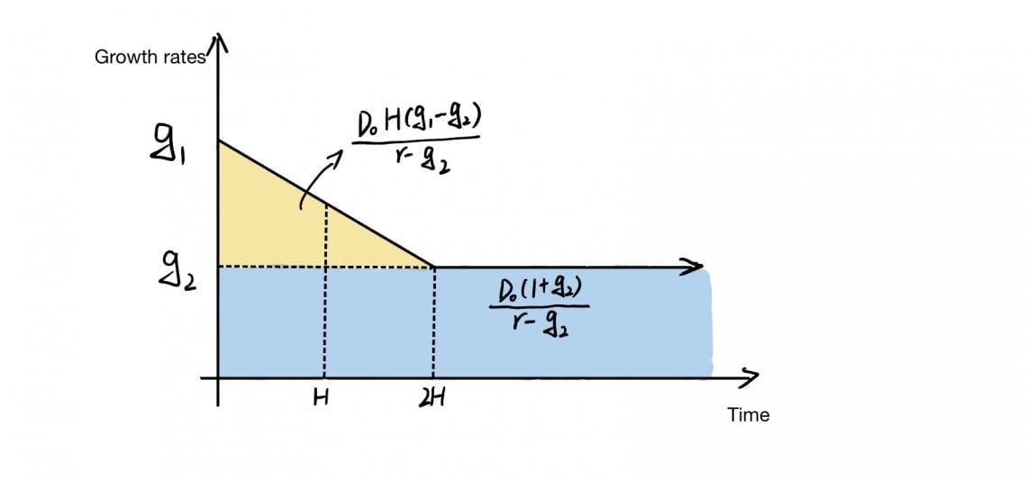
In the image of the model, the growth rate initially starts at a high growth rate, g1, which will decrease linearly as time passes. When the growth rate reaches the terminal growth rate, g2, the drop stops and will be stabilized at g2 permanently.
H-Model vs. Two-Stage Model
With the basic concept of the H-model in mind, we can take a further look at the difference between the H- and two-stage models.
Before comparing, let's briefly talk about what a two-stage model is. For example, the H-model of equity valuation is a two-stage rather than a model based on two cash flows.
We know that, in the first stage of the model, there is a high and ever-decreasing growth rate, while we usually assume a constant growth rate in the second stage.
Let’s say we aim to value a company whose first stage has an unstable initial growth rate and a stable growth rate in the second stage. We will assume that the company pays the dividend in the same way, allowing us to use a two-stage model.
The formula for this model is:

The output of this model interprets that:
1. The company is undervalued when the market price (MP) is less than the model’s output, meaning that our estimated growth rates are higher than the current value assumes.
2. The market expects growth rates to increase faster than we expect when the MP of a company is higher than the model output.
There are, however, several defects of the two-stage model:
I. Errors may occur when estimating the length of the first stage, which could lead to undervaluation or overvaluation of the stock
II. Assuming a direct jump in growth rate
III. Usage and capability are limited
Considering these shortcomings, we have other models that reduce estimation error, like the H-model. However, since the model is a modified two-stage DDM, what are the differences between the properties of these two models?
| H-Model | Two-Stage Model |
|---|---|
| Assume an increasing or decreasing growth rate in the initial stage and assume it will be constant in the second stage. | Assume a constant growth rate in the initial stage. |
| The growth rate declines/inclines linearly. | Cliff jumps exist in the growth rate. |
Both models assume the dividend payout ratio and cost of equity are constants, which may lead to estimation errors. Considering this flaw, why do we still choose this model? What are the advantages?
Compared with the two-stage model, the advantages of the model are:
- Consistency: Dividends remain steady over a long period.
- No bias: The definition of dividend payment is recognized universally.
- Sign of maturity: When the company reaches its peak maturity, shareholders receive dividends yearly.
The model allows for a changing dividend growth rate over time, providing an easier way to estimate the results than popular three-phase models. In addition, simple steps can yield a direct solution for the discount rate.
This model works well when estimating the stock value of a company with an initially high growth rate and a high probability of declining as the business gets larger.
The following video gives an example of how the H-Model is used:
To create an H-model, we can follow the four steps below:
- Establish the dividend amount
- Establish the growth rates and duration of time
- Establish the cost of equity capital or required return
- Plug into the formula
Now, let’s look at an example.
H-Model – UPS Example
At the end of 2018, UPS paid $3.64 per share dividends. UPS also planned to continue buying its shares from shareholders to return cash over three years.
A net share purchase of $1.566 billion was made in 2018, while others held 870 million shares. In other words, UPS returned $5.44 per share of cash to investors in that year.
For calculations, we assume the revenue growth rate is 7.7% on average over the three years, and the long-term growth rate is stable at 10% in the future ten years. We will use 9% to approximate historical stock market returns.
In this example, the dividend amount is $5.44 per share; short- and long-term growth rates are 7.7% and 9%, respectively, and the required return is 9%.
Then, we plug this information into the model formula:

Hence, the value of each share is $118.95.
Inputs, such as the discount rate, the growth rate, and the year of use, can greatly impact the accuracy of the model’s calculations. The entire model improves when we provide a reliable cash flow estimation to shareholders.
All in all, the H-model is a major advance in stock valuation. It solves the problem of sudden declines in growth rates assumed by other models. However, it still provides only one estimate, albeit better than the dividend discount model in terms of stock valuation.
H-Model FAQs
The two-stage dividend discount model considers two stages of growth. Instead of a model based on two cash flows, this approach to equity valuation is a two-stage model.
The first stage will generally have a high, slowly-decreasing growth rate, while the second stage is usually considered to have a stable growth rate.
In finance and investment, the discounted dividend model (DDM) is a method of valuing a company's stock based on the sum of all the company's future dividend payments, discounted to its present value.
It was first introduced in John Burr Williams' 1938 book “The Theory of Investment Value,” which was published 18 years before Gordon and Shapiro proposed the dividend discount model.
No, the dividend discount model, while still valuating a company, focuses on the present value of all future dividends. On the other hand, a discounted cash flow analysis focuses on the present value of all future cash flows.


or Want to Sign up with your social account?