Empirical Rule
Virtually every piece of data will fall within three standard deviations of the mean


What Is The Empirical Rule?
The empirical rule, in statistics, states that, for a normal distribution, 99.7% of all observations should fall within three standard deviations of the mean.
It is also known as the three-sigma rule and the 68-95-99.7 rule because it predicts that:
- 68% of all observations will fall within one standard deviation of the mean.
- 95% of all observations will fall within two standard deviations of the mean.
- 99.7% of all observations will fall within three standard deviations of the mean.
- The empirical rule applies to normal distributions, indicating that approximately 99.7% of data falls within three standard deviations of the mean.
- It follows the 68-95-99.7 rule, meaning 68% of data falls within one standard deviation, 95% within two, and 99.7% within three.
- It's crucial to calculate standard deviation, which measures data spread around the mean.
- The rule is useful for estimating probabilities and risk management in fields like finance and business when dealing with normal distributions.
Empirical Rule—Normal And Non-Normal Distributions
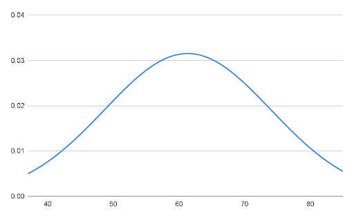
A normal distribution is often referred to as a bell curve because it looks like a bell, where more observations are concentrated around the mean instead of farther away (there is no skew).
On the other hand, if the observations are far away from the mean, a distribution will be considered non-normal, and skewed to the left or right. This will cause the rule to not hold because a distribution must be normal, where the mean is equal to the median, which is equal to the mode.
Below is an illustration of a bell curve or normal distribution.
If a distribution is skewed to the right or left, the mean, median, and mode will not be equal.
In a skewed distribution:
- 68% of the observations will NOT fall within one standard deviation of the mean;
- 95% of the observations will NOT fall within two standard deviations of the mean; and,
- 99.7% of the observations will NOT fall within two standard deviations of the mean.
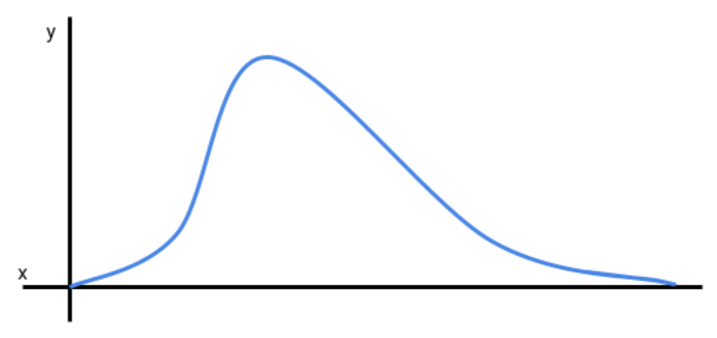
Below is an illustration of a positively skewed distribution. Notice how large values are pulling the distribution to the right. In this distribution, the rule will not hold.
Empirical Rule—Standard Deviation
To understand the empirical rule, it is important to understand what standard deviation means.
The standard deviation measures the dispersion of a given data set, i.e., how spread apart the numbers are from the mean of the data set. It helps paint a better picture of the distribution, in relation to its mean.
Three steps must be taken to calculate the standard deviation:
- Calculate the mean (average) of the data set
- From the mean, calculate the variance
- Take the square root of the variance to arrive at the standard deviation
Using the Empirical Rule
One of the benefits of using the empirical rule is that it can quickly be applied to a normal distribution to estimate the probability that an observation will fall within +/- one to three standard deviations of the mean with some precision.
In order to use the concepts of the rule, the distribution must be a normal distribution, that is 68% of the observations will fall within +/- one standard deviation from the mean of the distribution.
Let’s assume a pharmacy would like to anticipate the number of flu cases, within one standard deviation of the mean, so they can properly stock the shelves with medicine.
The pharmacy has determined that the historical mean for the flu during the flu season is 9, with a standard deviation of 3. The distribution is also normally distributed.
The pharmacy can now estimate the range for one standard deviation by adding the standard deviation to the mean, and, separately, subtracting the standard deviation from the mean.
The range for one standard deviation is provided below:
1 : (9 - 3) to (9 + 3) = 6 to 12
The pharmacy can anticipate with 68% accuracy that the probability of flu cases in the upcoming flu season will be between 9 to 12 cases (within one standard deviation of the mean).
Empirical Rule In Finance
In finance, the empirical rule can be used to forecast returns with some precision. But the return series (data set) being analyzed must be normally distributed, and the standard deviations must be known.
If it is a normal return series and the standard deviations are known, then an analyst can predict that:
- 68% of returns will be within one standard deviation of the mean
- 95% of returns will be within two standard deviations of the mean
- 99.7% of returns will be within three standard deviations of the mean
If the return series isn’t normally distributed (non-normal distribution), then forecasting future returns may not be as simple, and the rule cannot be applied.
The empirical concept is primarily used by traders, especially quantitative traders.
Examples of its use in finance include as part of mean-reverting strategies or Monte Carlo simulations. Another use of the concept, in finance, is for risk management.
For example, VaR (Value at Risk) utilizes the empirical probability to find the 1% or 5% risk of maximum loss on any given trading day. It is also used in stress tests to understand the impact of tail events on the company’s solvency.
Empirical Rule Example
Let’s assume the volume of shares traded of a renewable energy stock, over the last twelve months, are normally distributed, with an average daily volume (ADV) of 2 million shares, and a standard deviation of 1.2 million shares.
An investment analyst for a pension fund would like to know the probability that more than 3.2 million shares will be traded in a day.
To calculate the probability, the analyst will use the ADV, or the mean, of 2 million shares; the standard deviation of 1.2; and the fact that the trading volume over the last twelve months is normally distributed.
Given the fact that the trading volume is normally distributed, the analyst can apply the empirical concept. They know that:
- 68% of returns will be within one standard deviation of the mean
- 95% of returns will be within two standard deviations of the mean
- 99.7% of returns will be within three standard deviations of the mean
Since the analyst knows the mean and standard deviation of the distribution, they can calculate +/- standard deviation ranges for each standard deviation by adding the standard deviation to the mean, and, separately, subtracting the standard deviation (SD) from the mean.
- 1 SD: (2 - 1.2) to (2 + 1.2) = 0.8 to 3.2
- 2 SD: [2 - (1.2 x 2)] to [2 + (1.2 x 2)] = -0.4 to 4.4
- 3 SD: [2 - (1.2 x 3)] to [2 + (1.2 x 3)] = -1.6 to 5.6
Now that the analyst has the ranges, they can determine that 32% of the observations are outside of one standard deviation from the mean (less than 0.8 million and more than 3.2 million shares).
This is because, in a normal distribution, 68% of all observations will fall within one standard deviation from the mean, which means 32% will be outside of this range.
Since half of the observations will be more than 3.2 million shares (32% divided by 2), the analyst can expect that no more than 16% of the average daily trading volumes will be greater than 3.2 million shares.

Free Resources
To continue learning and advancing your career, check out these additional helpful WSO resources:


or Want to Sign up with your social account?