CONCATENATE Function

What is the CONCATENATE Function?

The CONCATENATE function in Excel can join two or more text strings, numerical values, or formulas in Excel.

The easiest way to understand the concept of concatenation is through a Ponzi scheme. When a fraudulent person begins such practices, he expects the initial investors to recommend the scheme to others forming a chain of investors.

The first initial investor expects at least three people to join him, those three expect at least nine people to join(three each), and so on.

We see that each person connects other people to the Ponzi scheme. The CONCATENATE function works similarly, but the difference here is that it connects different text values in Excel.

It is one of the most used functions in Excel and offers the user much more flexibility in terms of what result to return based on combining multiple formulas.

In this article, we will see the function, its syntax, and a couple of examples to understand it better.

CONCATENATE function Formula

The function is categorized as a Text function connecting two or more text strings or even formulas in Excel.

However, since a newer version of CONCATE replaced the function, you will find it under the Compatibility section for backward compatibility in Excel.

What’s different in the newer version?

It will directly combine the values from multiple ranges without referencing each cell in the formula. Well, more on that later, but first, let’s understand the function.

Suppose you have the two text strings as ‘abc’ and ‘def’; then the formula will give you the result as ‘abcdef.’ As you can see, the function combines both text strings to return the result as one.

The syntax for the function is,

=CONCATENATE(text1,[text2]...)

where,

• text1 - (required) the first text string, numerical value, or the cell reference
• text2 - (optional) the second text string, numerical value, or the cell reference

How to use the CONCATENATE Function in Excel?

If you have been reading many of our Excel articles, we usually tell you one thing - “You can use the function in two different ways - from the function’s library or as a worksheet formula.”

We will contradict that statement and say there are three methods to use the function.

Method #1: From the function’s library

To use the function from the library, please follow the steps below:

1. First, select the cell in which you expect the result.
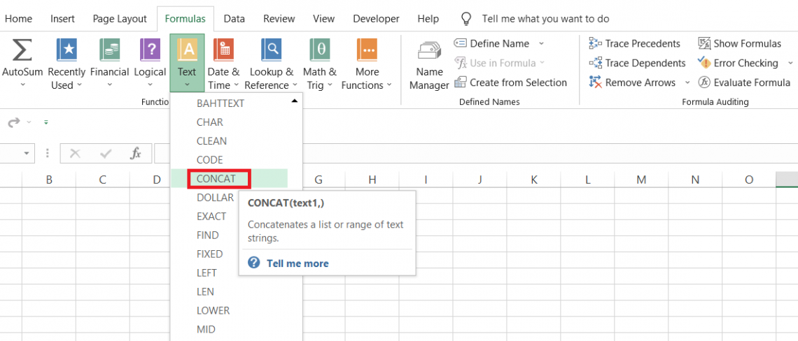
2. Click on Formulas > More Functions > Compatibility > select the CONCATENATE function from the drop-down menu.
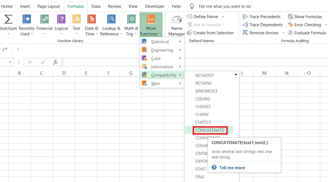
3. We will input the text strings, numbers, or cell references in the dialog box as illustrated below, which displays the result:
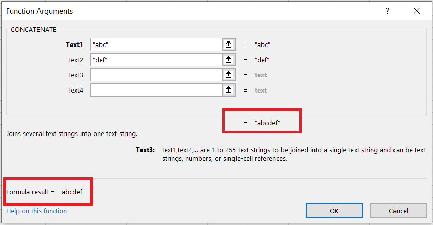
4. Once you click on Ok, you get the same result in the selected cell.
5. Although the method is simple and easy to understand, it is not the best in terms of efficiency. 
   However, if you are just a beginner who has just started this magical journey of conquering Excel, then you should check the rest of those functions from the library.

Method #2: As a worksheet formula

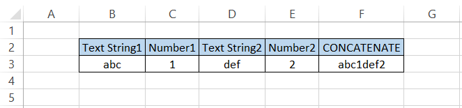
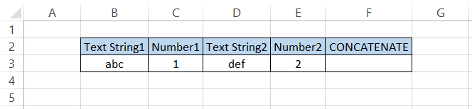
The second method uses the function as a worksheet formula. For example, suppose you have the data as illustrated below:

We will use the formula =CONCATENATE(B3,C3,D3,E3) in cell F3 by referencing individual cells, which gives us the result as ‘abc1def2.’

Although the cell connects the text strings, the function's only downside was that we had to reference each cell in the formula individually. However, that has been overcome using the newer CONCAT version.

Method #3: Using the ‘&’ symbol

If you feel that typing in the formula or using the function from the library might take a lot of time, you can directly combine the text strings using the ‘&’(ampersand) symbol.

Suppose the data looks as below:

We will begin with an equal sign and reference each cell separated by the ampersand symbol(&) such that the formula is =B3&C3&D3&E3, which gives a similar result:

This method is often useful in complicated formulas when you are concatenating multiple values together in, let’s say, a VLOOKUP or an INDEX MATCH formula.

CONCATE Function Example

It doesn’t make sense if we see the same examples again. So let’s take it one step further and see how you can use the function or the concept of concatenation in complicated formulas.

First, the more compact formula is, the easier it is to understand, which is why we will mostly use the ‘&’(ampersand) symbol and CONCATENATE occasionally in the formulas.

There is nothing wrong with either method, but we prefer the former since it is easier to understand while checking errors and is accessible.

We will see the complicated formulas based on lookup formulas, such as VLOOKUP, and logical formulas, such as AND, OR, NOT, etc. However, there is no limit to where you can use concatenation unless it gives you an error.

Example #1: CONCATENATE with VLOOKUP

If your VLOOKUP table consists of values that are a combination of two or more values, then the function works well to get the desired results.

Suppose you have the student’s test scores table on one spreadsheet and their status on another spreadsheet, whether they have passed or failed.

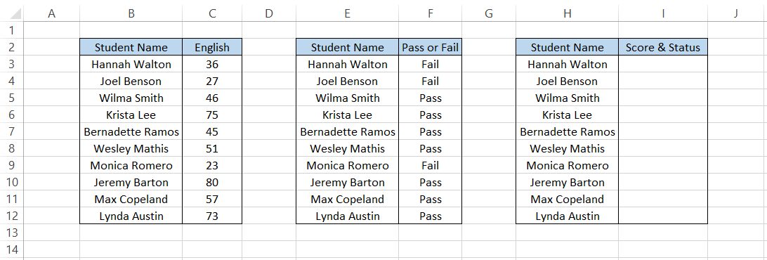
However, you want the test scores and the status together on the third spreadsheet in a single column.

In this case, we will use the formula =VLOOKUP(H3,$B$3:$C$12,2,FALSE)&" - "&VLOOKUP(H3,$E$3:$F$12,2,FALSE) in cell I3 and drag it down till cell I12, which gives the result:

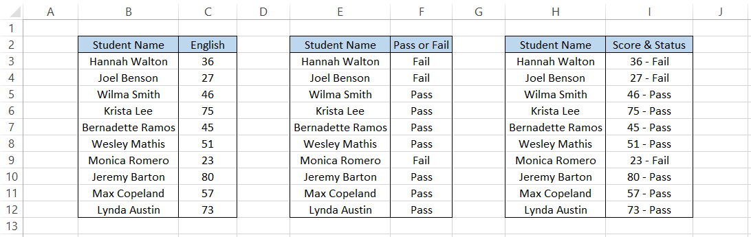
The values are combined and separated by the delimiter ‘-’ in column I.

Alternatively, you can also use the formula =CONCATENATE(VLOOKUP(H3,$B$3:$C$12,2,FALSE)," - ",VLOOKUP(H3,$E$3:$F$12,2,FALSE)), which gives us a similar result, but you can see the difference in how to complicate the formula starts to look.

It's not the result you can combine, but even the lookup_value argument in the VLOOKUP formula.

Suppose you have the ‘Student Name’ and the English test scores in one workbook while the other workbook consists of first names and last names along with the test scores you need to import.

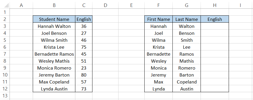
Here, you can combine the first and last name using the concatenating ‘&’ symbol, which will ultimately pull in the English test scores for the respective students.

The formula will be =VLOOKUP(F3&" "&G3,$B$3:$C$12,2,FALSE), which gives the result in column H as

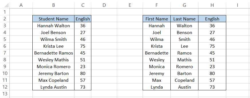
We first combine the first and last names but let’s not forget to separate those two strings by a space character represented between the quotation marks. Had you not mentioned the space character, you would get the #N/A Error.

Example #2: Along with Logical functions

Some of the most widely used logical functions are AND, OR, IF statements, etc., which return the result as TRUE if the criteria are fulfilled and FALSE if the criteria are not fulfilled.

Let’s say there is a text string that combines two or more values. You want to compare whether those text string combinations match the complete version.

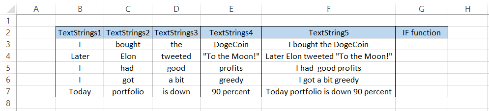
Here, we can use the IF statements to compare the combination of the text strings in range B3:F7 to the text strings in column F.

The only character we will input additionally will be the space character between each text string. If any other characters are missing, the function will return the result as FALSE.

The formula will be =IF(B3&" "&C3&" "&D3&" "&E3=F3,TRUE,FALSE) in cell G3, which we will drag to cell G7, giving you the result:

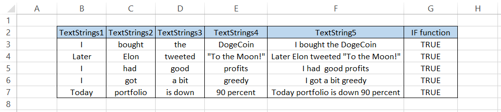
We combined the text strings in columns B, C, D, and E, separated by the space characters, and then compared them to the text strings in column F using the logical operator, i.e., the equal sign(=).

Since all the combinations were equal to strings in column F, we get the evaluation result as TRUE in all the cells in column G.

These are just a few examples where you can use the function or the ampersand symbol (&) to combine text strings or numerical values. Still, in reality, the sky is the limit for the function.

CONCATENATE vs. CONCAT function

The CONCAT function was introduced in Excel 2019 and has been present in all the subsequent versions and Excel 365.

Both functions work on the same principle, so what is the difference? As we already know, Microsoft doesn’t make any changes without reason. All the newer versions are based on the same motive - improving efficiency for Excel users.

We previously saw how to individually reference the cells in the formula using the function or even the ampersand symbol(&) to combine two text strings.

The CONCAT function, on the other hand, combines the text strings or numerical values directly from the referenced range of cells.

The syntax for both functions is similar as

=CONCAT(text1,[text2]...)

where,

• text1 - (required) reference to the cell or range of cells consisting of text strings or numerical values.
• text2 - (optional) reference to the cell or range of cells consisting of text strings or numerical values.

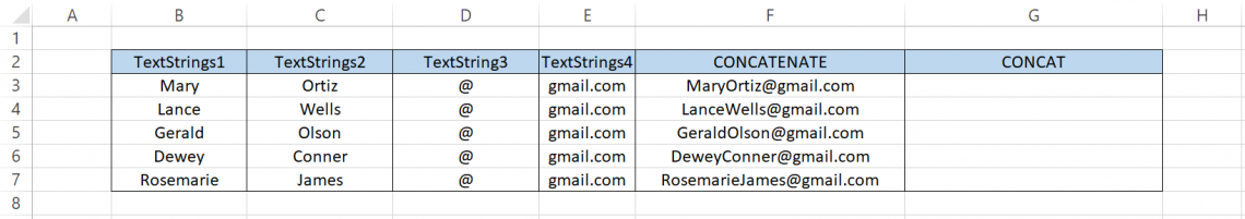
To understand how easy the function makes concatenating multiple text strings, let’s see a simple example. Suppose you have the data as illustrated below:

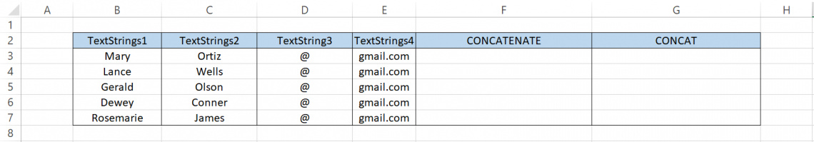
The four columns consist of the first names, last names, @ symbol, and ‘gmail.com’. We want to generate the email ids for the individual people using either function.

Firstly, by using the formula =CONCATENATE(B3,C3,D3,E3) in cell F3 and dragging it down till cell F7 gives the result:

Another formula you can use is =B3&C3&D3&E3, giving us the same result. But you see the issue, right? What if we had 200+ text strings that needed to be combined?

Reference each text string in the formula would take a lot of time. Well, that’s where the CONCAT function comes in. 

We will use the formula =CONCAT(B3:E3) in cell G3 and drag it down to cell G7, giving you the result:

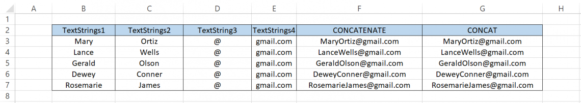
Wasn’t that easy? Just a single argument allows you to input text strings from multiple cells. If that’s not enough, the function has been upgraded to include a total of 32,767 characters before the function returns the #VALUE! Error as compared to CONCATENATE’s 8,192 characters.

Opposite of CONCATENATE

Right, we combined a couple of text strings. Still, there could be instances when we want to separate the components of the text strings into different cells. 

What would you do?

There are several methods with which you can return results opposite to the concatenation, the most prominent is the Text to Columns tool.

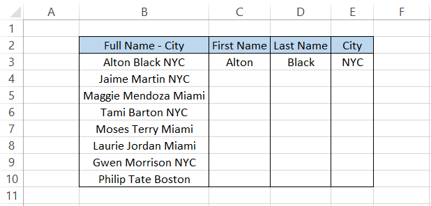
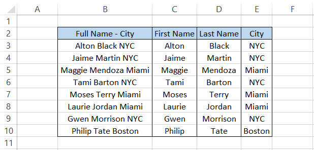
Suppose you have the text strings consisting of the full name followed by the city where that person lives.

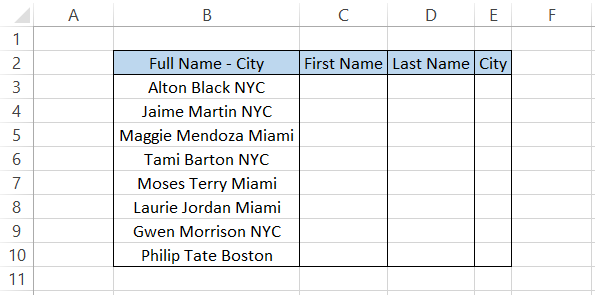
An important point to remember is that all those substrings are separated by a common ‘delimited,’ which is the space character.

To separate the substrings, we will select the range B3:B10 > Data Tab > Select the Text to Columns tool, which opens the dialog box as illustrated below:

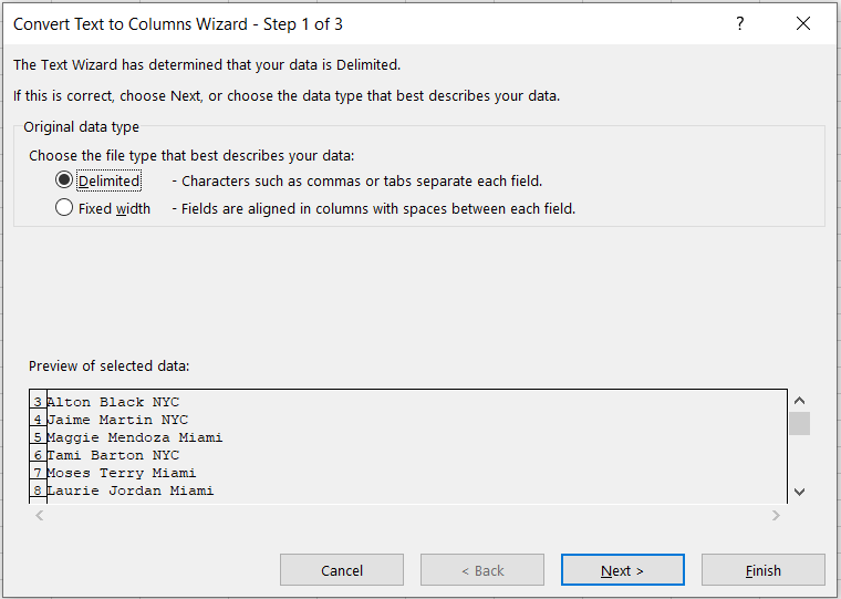
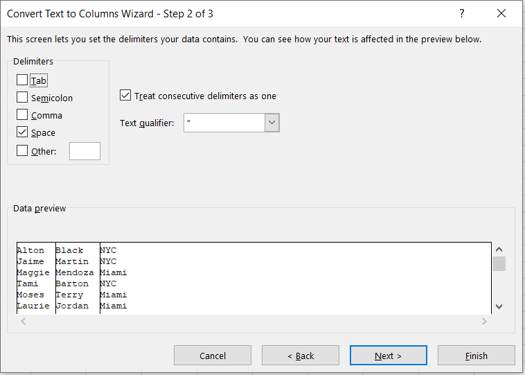
We will click on Next and select the delimiter as the space character. Additionally, you can select multiple delimiters by just inputting the tick mark on the check box for each of those delimiters. Once done, click on Next.

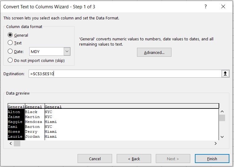
Finally, we will input the destination of the cell range in which we expect our result. Of course, we can also change the other formats, such as Date.

Once you click on Finish, sometimes you might get a warning error such as:

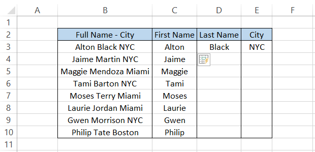
Just click on Ok, and you will find the distinct values in the selected ranges, i.e., C3:E10.

Another method is using Flash fills. Again, the substrings must be separated by the delimiters, which is the space character in our case. First, we type in the substring separate in each of those columns.

Now, all you need to do is press the keyboard Alt + E key in each of those cells containing the substring. For example, select cell C3 and press the Alt + E key. You will get the result:

Similarly, you can choose the D3 and E3 cells separately and press the Alt + E key to give the separated first name, last name, and the city in which they live.

There are other complicated formulas, such as a combination of MID, RIGHT, or LEFT functions and SUBSTITUTE and TRIM, that you can use to separate substrings.

The only thing is - it won’t be covered in this article. So, to keep this article plain and simple, we have covered those examples in the articles of the mentioned functions.

Once you have understood the concept for the function, you can head over to the more complex formulas in those text functions!

Researched and authored by Akash Bagul | LinkedIn

Reviewed and edited by Parul Gupta | LinkedIn

Free Resources

To continue learning and advancing your career, check out these additional helpful WSO resources:

• TRUE Function
• UPPER Function
• VAR.P Function
• WORKDAY Function
• XIRR Function