TRUNC Function

What is the TRUNC Function?

The TRUNC function in Excel can remove the decimal digits from a number to truncate it to an integer.

Please make sure the function's name is distinct from the car's storage compartment. Although both sound similar, they perform different tasks.

We have seen a lot of functions that truncate all the digits after the decimal point on their own when you input fractional numbers; finally, we will see a part that gives us control over how many numbers to truncate.

First, let's understand the term 'truncate.' You can say it's a fancy term that ignores all the digits after a specific number. A question might come to your mind," Don't we have functions similar to that"?

Yes, we do. Some of those are ROUNDUP, ROUNDDOWN, ROUND function, etc., limiting a number to a certain number of digits after a decimal point. However, they do round up the value in the process.

The TRUNC function, on the other hand, does not round a number but relatively completely removes or ignores the digits after the decimal.

In this article, we will see the TRUNC function, its syntax, and a couple of examples to understand it better.

Understanding the TRUNC Function

The TRUNC is categorized as a Math and Trigonometric function that removes the 'n' number of decimal digits from a number to return a truncated number.

For example, if you have the number 47.8946 and need to truncate it to an integer, then using the function will return the result as 47.

Another beauty of the function is that it gives control to the Excel user over how many digits to truncate after the decimal.

Even though the argument is optional, you can input a number corresponding to the digit after the decimal, after which all the numbers get truncated.

For example, if the number is 47.8946 and you need to remove all the digits after the second digit after the decimal, the function gives the result as 47.89.

The syntax for the TRUNC function is

=TRUNC(number,[num_digits])

where,

• number - (required) the number which will be truncated
• num_digits - (optional) the number of digits after the decimal, which will be removed from the numerical value. The default value is 0, which returns the integer value.

The function was introduced in Excel 2003 and has been present in all the subsequent versions.

How to use the TRUNC Function in Excel?

Since the syntax for the function is easy to understand, using the process makes it even easier.

To use the function, you must select the cell where you need the result and type in the function name followed by the arguments inside the parentheses.

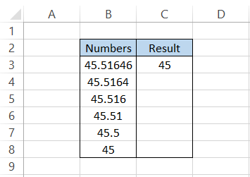
For example, suppose that you have numbers in Excel, as illustrated below:

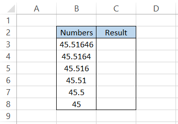
Using the formula =TRUNC(B3) in cell C3(yes, we will ignore the num_digits argument for now) gives us the integer value 45.

What if we truncate the numbers based on the num_digits argument?

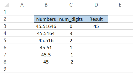
As you can see, we have created an additional column consisting of the num_digits argument. There are also negative values for the num_digits argument, so it will be interesting to see what result we get for those values.

The formula that we will use is =TRUNC(B4, C4) in cell D4 and drag it down till cell D8 which gives the result:

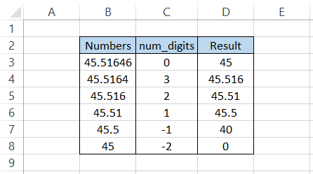
All the digits specified after the num_digits argument are removed from our number, as in the mixed results illustrated above. There are a couple of unique issues as well; when we reference an opposing num_digits argument, the number rounds down toward zero.

So there is some similarity to rounding functions; however, the general idea for the part is still to remove the digits until nothing is left of the given number.

TRUNC Function Examples

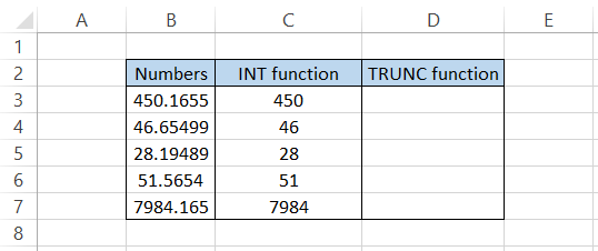
As we said earlier, the function works only with numbers or values related to numbers, such as date and time. For example, suppose that you have numbers in Excel, as illustrated below:

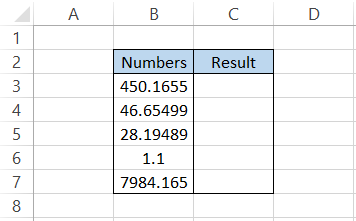
To limit them all to integer values, we will use the formula =TRUNC(B3) in cell C3 and drag it down to cell C7, which gives the result:

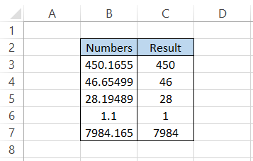
Remember that since we do not use the num_digits argument, the default value selected is zero, which ultimately returns the integer value.

If you were to limit the numbers to two digits after the decimal, we would use the formula =TRUNC(B3,2) in cell C3 and drag it down to cell C7, which gives:

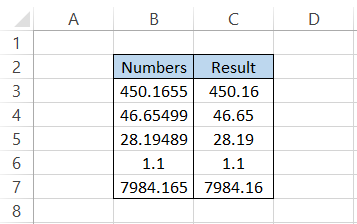
Except for cell B6, which has just one digit after the decimal, all the numerical values have limited themselves to two digits after the decimal. Therefore, the function returns the same number if there are no numbers, like in cell B6, as opposed to our num_digit argument.

You probably won't be using the function on time and date values, but it definitely won't hurt to see the effect function has on those values.

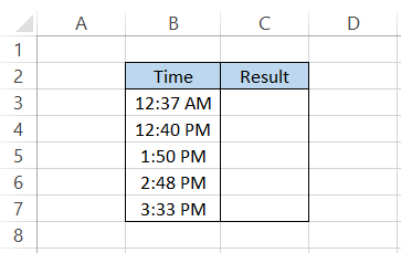
Suppose that you have the time values in Excel as illustrated below:

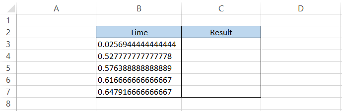
We do need to remember that time is stored as decimal numbers while dates are stored as serial numbers in Excel. So if you press the Ctrl + ~ key on the keyboard, the decimal number equivalent for the time would be:

When you use the function and limit those time values to two decimal digits using the formula =TRUNC(B3,2), we get the result:

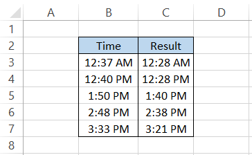
If you change the format of the results in column C to 'Numbers' form, we get the following:

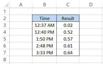
As you had previously seen, the decimal equivalent of the time when we change the format from 'time' to 'numbers', we get the first two digits after the decimal as our result. So I hope all the things are correlating and making sense!

TRUNC vs. ROUND function

As we have previously said, the TRUNC function does not 'round' a number in Excel. Instead, it limits a numerical value to 'n' digits after the decimal. The function rounds the numbers toward zero if you use negative integers for num_digits.

However, on the other hand, the ROUND function is categorized as a Math and Trigonometric function that will round up a number to a specified number of decimal places.

The function has the ability to both: round up the number as well as round down based on predefined criteria.

The criteria are such that if the succeeding 'nth' digit to the right lies between five and nine, then the function rounds up the number, whereas if the succeeding 'nth' digit is between zero and four, then the number rounds down.

For example, if you have 17.3148 in a cell and use the function to round up the number to one decimal digit, we would get the result as 17.3 since the second digit after the decimal lies between zero and four.

If the same number was 17.3848, the rounded value would be 17.4 since the second digit after the decimal is between five and nine.

The syntax for the function is

=ROUND(number,num_digits)

where,

• number - (required) the number which will be rounded to specified decimal places
• num_digits - (required) the number of decimal places to which you want to round the value.

Note: The num_digits argument can take negative, zero, or positive opinions to return a rounded value.

Let's see an example to understand the difference between the result that the TRUNC and ROUND function respectively returns.

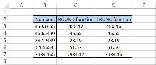
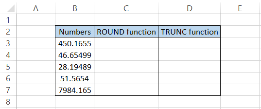
Suppose that you have numbers in Excel as illustrated below:

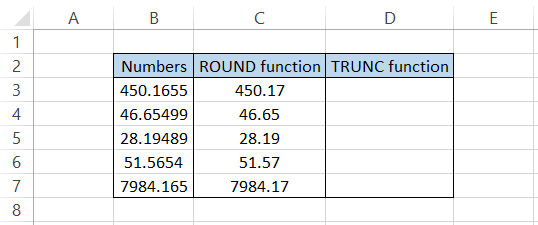
Let's say we limit the numbers to two digits after the decimal for both cases. The formula that we will use in cell C3 will be =ROUND(B3,2) which gives the result of 450.17

Dragging down the formula till cell C7, we get:

Similarly, in cell D3 we will use the formula =TRUNC(B3,2) and drag it down till cell D7, which gives the result:

You would notice that whenever the number rounds up, i.e., if the succeeding 'nth' digit lies between five and nine, we get a contrasting result for both functions.

However, if the digit lies between zero and four to round down the number, both functions yield the same result.

Yes, the result matters while working in Excel. So if you want to round a number, you can use the ROUND function or shift to using TRUNC to remove up to 'nth' numbers altogether.

A task for you - How would other number rounding functions, such as MROUND, ROUNDUP, ROUNDDOWN, etc., behave compared to TRUNC? 

TRUNC vs. INT Function

When you do not input the num_digits argument inside the function, it will return the integer value for that number.

What is the other alternative to get those integer values?

Well, it's none other than the INT function, which rounds a given numerical value to its nearest integer.

The INT function works precisely similarly to when you ignore the num_digits argument in the TRUNC function.

For example, if you have the number 17.481 and use the INT function, you will get the result 17. Similarly, if the number is 2848.1, the expected result would be 2848.

All the digits after the decimal point are ignored to return the integer value for the given number.

The syntax for the INT function is

=INT(number)

where,

number - (required) is the number that will be rounded down to its integer value.

To understand the similarities and dissimilarities between both functions, let's see an example. Suppose that you have numbers in Excel as illustrated below:

By using the formula =INT(B3) in cell C3 and dragging it down to cell C7, we get the result:

Similarly, by using the formula = TRUNC(B3) in cell D3 and dragging it down to cell D7, the result is:

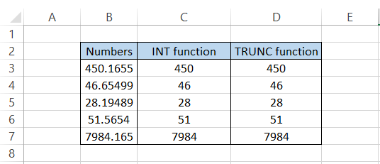
As you can see, both functions yield a similar result when the objective is to get the integer for the numerical value.

Researched and Authored by Akash Bagul | Linkedin

Reviewed and Edited by Raghav Dharmarajan