Econometrics

What is Econometrics?

Econometrics is a specialized field that employs statistical and mathematical methods to examine and validate economic relationships and analyze economic data.

It was pioneered by Lawrence Klein, Ragnar Frisch, and Simon Kuznets. All three of them received a Nobel prize for their contribution. 

The econometric relationship shows the random behavior of relationships that are usually not considered in economics and mathematical formulations. Often, econometric methods are used in areas like geoscience, agriculture science, etc.

To break it down further, econometrics utilizes statistical methods adapted to address economic issues. These adapted methods, referred to as econometric methods, are primarily used to understand stochastic relationships—relationships with inherent randomness.

To break it down further, econometrics uses statistical methods by adapting them to economic issues. These adapted methods, referred to as econometric methods, are primarily used to ascertain stochastic relationships.

The two major branches of econometrics are:

1. Theoretical econometrics: Concerned with the development of appropriate methods for measurement of economic relationships, which are not meant for controlled experiments conducted inside the laboratories and are specifically developed for the analysis of non-experimental data.

2. Applied econometrics: Concerned with the implementation of econometric methods to particular branches of problems and economic theories. This implementation involves the application of the tools of econometric theory to the analysis of economic phenomena and forecasting economic behavior.

Aims of Econometrics

The main aims of econometrics are:

1. Formulation and specification of econometric models

Econometric models are formulated in an empirically testable form. Several economic models lead to the derivation of econometric models. Such models vary from each other because of the different functional forms used.

2. Estimation and testing of models

The parameters of the models formulated are estimated concerning the observed data set, and they are tested for their suitability. Unknown parameters of the model are given numerical values using various estimation procedures.

3. Application of models

The models are used for policy formulation and forecasting. Both these aspects are an essential part of policy decisions. Forecasts allow policymakers to look at the suitability of the fitted model and re-adjust relevant economic variables.

Types of Econometric data

1. Cross-sectional data

This type of data is collected by observing subjects like firms, individuals, countries, regions, etc., at one point or time.

Analysis of cross-sectional data generally comprises a comparison of differences between selected subjects without having regard for any difference in time.

For example, to measure the current obesity level of the people in a population, 2000 people are randomly selected from the population. Then, their height, weight, and the percentage of obesity in that sample are calculated.

In a rolling cross-section data, the presence of an individual in the sample and the time at which the individual is included in the sample is determined randomly. 

Cross-sectional regression is performed using this data type.

For example, the inflow of foreign direct investment could be regressed on exports, imports, etc., in a fixed month.

2. Time series data

It is a collection of observations obtained through repeated measurements over time. When plotted on graphs, these observation points are always plotted against time on one axis.

Since our world gets increasingly instrumented, systems are seen constantly emitting a relentless stream of time series data. Time series data can be observed anywhere and everywhere.

Some commonly observed examples are weekly weather data, health monitoring, temperature readings, logs, traces, stock exchange, etc.

Time series data can either be measurements gathered at regular time intervals or measurements gathered at irregular time intervals. It is generally seen in bool, string, float64, and int64.

3. Pooled- cross-sectional data

These types of data sets consist of the properties of both time series and cross-sectional data sets. Here we take random samples in different periods of different units often used to look at the impact of policies or programs.

For example, the household income data of A, B, and C individuals are taken for the year 2000, and for D, E, and F, it is taken for 2010. The same data is taken for different households in different periods.

4. Panel data

Also known as longitudinal data, contains data of different cross-sections across time. In this method, observations are collected at a regular frequency. 

Panel data consists of more information, efficiency, and variability than any other data type. It can model both the common and individual behaviors of groups. 

Gross domestic product across multiple countries, unemployment across different states, and currency exchange rate tables are all examples of panel data. 

Econometric methods

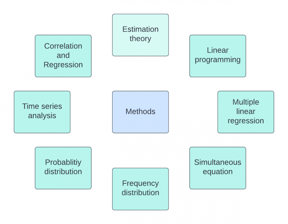
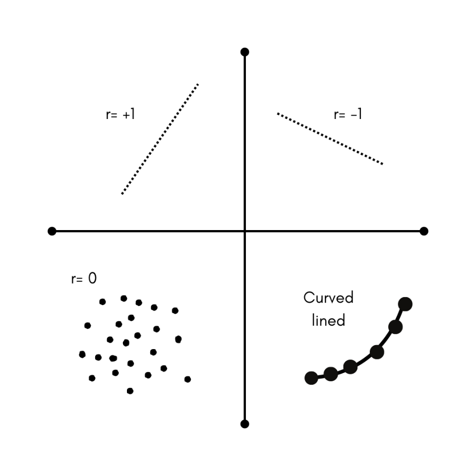
1. Correlation and Regression

Correlation analysis is used to see the association between two continuous variables: one dependent and one dependent variable or two independent variables.

The correlation coefficient sample is estimated in correlation analysis, which ranges from -1 to +1. It quantifies the direction and strength of the linear relationship between two variables.

Two variables can be positively correlated, negatively correlated, and not correlated. Two variables that are not correlated would have a value of r = 0.

Regression analysis implies the determination of the relationship between the variables. The variables are y and x, where:

• The dependent variable (y) is the outcome variable or response variable 

• Independent variables (x) are risk elements. 

Linear regression is an approach for modeling the relationship between a scalar component and independent variables. 

It can be simple or multiple linear regression depending upon the number of independent variables.

Linear regression focuses on conditional probability and helps find out the best line that predicts y from x. 

A simple linear regression equation looks like this:

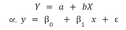
Here, Y is the dependent variable, and X is the independent variable.

Also, a and 𝛽0 are y-intercepts at time 0, 𝛽1 is the regression coefficient, and Ɛ is the error term.

2. Time series analysis

It is a specific way of analyzing a sequence of data points collected over an interval of time. Here, analysts record data points at consistent intervals rather than recording them intermittently or randomly.

Time series analysis requires a large amount of data to ensure reliability and consistency. In addition, it ensures that any trends or patterns discovered are not outliers and can account for seasonal variance.

It can be used for predicting future data based on historical data. 

Also, it facilitates the understanding of the underlying causes of trends and systematic patterns over a period of time.

Models constructed include :

• Classification of data that is identifying and assigning categories to the data.

• Curve fitting implies plotting data along a curve to study the relation of variables within the data.

• Descriptive analysis includes identifying patterns in the time-series data.

• Explanative analysis deals with understanding the data along with cause and effect.

• Explanatory analysis gives a visual format for understanding the data. 

• Forecasting means predicting future data. This is based on historical trends.

• Intervention analysis tells how an event can bring changes to the data set.

• Segmentation splits the whole data into segments to show the properties of source information.

3. Probability distribution

A probability distribution is “a statistical function that describes all the possible values and likelihoods that a random variable can take within a given range.”

A probability distribution is based on factors such as the mean of the distribution, standard deviation, skewness, and kurtosis.

On the one hand, skewness is a measure of symmetry. A data set or a distribution is said to be symmetric if both the left and right of the center point look the same. 

On the other hand, Kurtosis is a way to see whether the data is heavy-tailed or light-tailed compared to a normal distribution.

It can be used to create cumulative distribution functions that add up the probability of occurrences cumulatively. This function starts from 0n and ends at 100%.

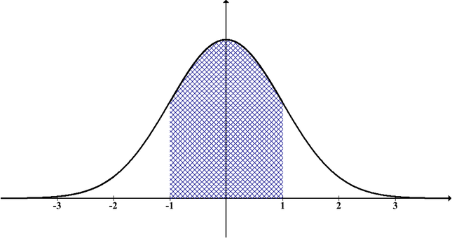
Some commonly used probability distributions are normal distribution, binomial distribution, Poisson distribution, and chi-square distribution.

Different types of distribution account for different purposes and variable generation procedures.

A normal distribution is mostly used for analysis as it is fully characterized by its mean = 0 and standard deviation =1. Also, its skewness is 0, and kurtosis = 3. This type of curve is the familiar, perfect bell-shaped, curved diagram.

4. Frequency distribution

“It is a tabular representation of data in which numerous items are arranged into different categories and mentioning properly the number of items falling in each category.” 

It is an important method of organizing and summarizing quantitative data. Grouped data is such a kind of data, whereas ungrouped data or raw data is the one that has not been arranged in a systematic order.

Representation can either be graphical or tabular. The number of observations displayed is of a given interval where intervals must be mutually exclusive and exhaustive.

The types of frequency distributions are grouped frequency distribution, ungrouped frequency distribution, cumulative frequency distribution, relative frequency distribution, and relative cumulative frequency distribution.

5. Simultaneous equations

This type of data generation process depends on more than one equation interaction together to produce the observed data. Here y variables in the system are jointly determined by the equations in the system. 

For instance, consider

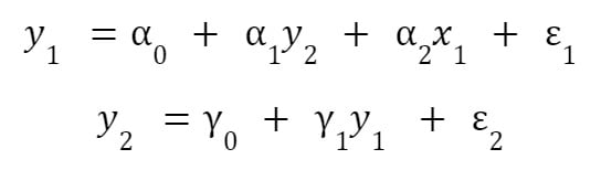
The first equation depends on the conventional variable x and a dependent variable. Similarly, the second equation depends on a dependent variable, y1.

Variables on the right-hand side of the equal sign are called exogenous variables, which are truly independent as they remain fixed. On the other hand, the variables appearing on the right-hand side, which also have their own equations, are endogenous.

Endogenous variables change their value as the equilibrium solution is ground out of the simultaneous equation model. 

They are endogenous as their value is determined within the system.

6. Multiple linear regression

It is a statistical technique that uses several explanatory variables to predict the outcome of a response variable. It is an extension of ordinary least squares regression.

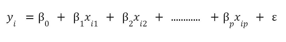
It is used when an analyst attempts to explain a dependent variable using more than one independent variable.

7. Linear programming

“It is a method to achieve the best outcome such as lowest cost or maximum profit in a mathematical model whose requirements are represented by linear relationships.”

Technological coefficients of linear programming are defined using linear regression.

8. Estimation theory

This theory deals with estimating the values of the parameters. These parameters are based on empirically measured data and consist of a random component.

The parameters are characterized by underlying physical settings. These settings suggest that the value of the parameter affects the distribution of the measured data.

The most common estimators are the Maximum likelihood estimator, Bayes estimator, method of moments, least square method, best linear unbiased estimator, and many more.

Researched and Authored by Parul Gupta | LinkedIn 

Free Resources

To continue learning and advancing your career, check out these additional helpful WSO resources:

• Brexit
• Contagion
• Fiat Money
• Gross National Product
• Quantitative Easing