ISTEXT Function
An Excel Information function that evaluates whether the referenced cell contains a text string or not and returns the result as TRUE or FALSE.


What is the ISTEXT Function?
The ISTEXT function is an Excel Information function that evaluates whether the referenced cell contains a text string or not and returns the result as TRUE or FALSE.
If there is a category of functions, wait... let me repeat it - “the category of simplest functions which are not only easy to understand but also quite easy to use then those fall under the Information function.”
The different types of Information functions you would find in Excel are ISLOGICAL, ISNONTEXT, ISNA, ISERROR, ISNUMBER, ISODD, ISEVEN…and finally, the ISTEXT function.
Each function evaluates the value and returns the result as TRUE based on its inbuilt criteria, which can be easily identified from the function name. For example, the ISODD function evaluates whether the given value is an odd number.
If it is, the function evaluates to TRUE, or it will return the result as FALSE.
Similarly, this article will examine the ISTEXT function, its syntax, and a couple of examples to help us better understand it.
- The ISTEXT function is an Excel Information function used to check if a value is text. It returns TRUE if the value is text and FALSE if it is not.
- The ISTEXT function is useful in scenarios where you need to determine if a value is text before performing certain operations or calculations.
- If the value is an error value (e.g., #VALUE!, #REF!, #DIV/0!), the ISTEXT function returns FALSE.
- The function is particularly useful in data validation and conditional formatting scenarios where you need to handle different types of data appropriately.
ISTEXT function Formula
The ISTEXT is categorized as an Information function that simply checks whether the given value is a text string and returns the result as TRUE.
The function returns the result as FALSE if the referenced cell does not contain a text string.
For example, if you have the text string as ‘Microsoft Inc,’ then the function will evaluate to TRUE. But, conversely, if the value is ‘69,’ the function evaluates the value as FALSE.
The syntax for the function is
=ISTEXT(value)
Where,
- value - (required) reference to the cell containing text string, numbers, logical values, errors, etc.
Note
You can reference any type of value inside the function or even hardcode it directly between quotation marks. However, the function only identifies text strings as the valid data type to return the result as TRUE.
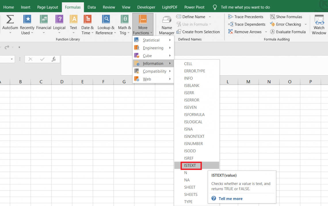
How to use the ISTEXT Function in Excel?
If any function needs more than two examples to explain, it is the INDEX MATCH combination. On the other hand, ISTEXT falls under the category of simpler functions since it comprises just a single argument.
This section will show an example of how the function works.
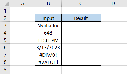
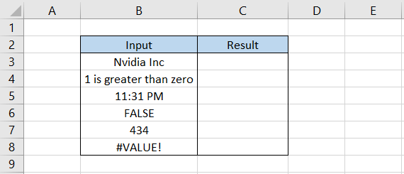
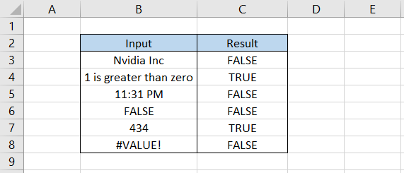
Suppose we have the data as illustrated below:
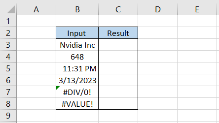
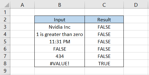
By using the formula =ISTEXT(B3) in cell C3 and dragging it down till cell C8, we get
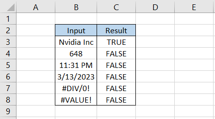
As you can see, the function evaluates to TRUE since we have the text string ‘Nvidia Inc’ in cell B3.
In other instances, we have number 648, time and date values of 11:31 PM and 3/13/2023, respectively, and error values. As none of these are closer to a data type as a text string, the function evaluates them as FALSE.
Combine the ISTEXT function with the IF function, enabling you to return two customized text strings for the result.
For example, the formula becomes
=IF(ISTEXT(B3)=TRUE,"It is a text string","Not a text string")
which gives the result:
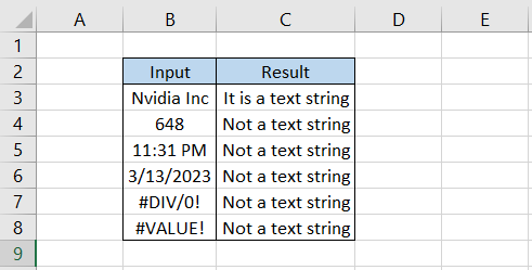
As expected, the function will return the customized text string as ‘It is a text string’ only for the value in cell B3.

ISTEXT Function Alternatives
Apart from ISTEXT, one can access several pieces of information from the function’s library or even directly type in the cell as a formula.
Some of those are ISNONTEXT, ISLOGICAL, ISFORMULA, ISERROR, ISNUMBER, ISBLANK, etc.
In this section, we will see and try to understand some of those information functions better.
ISNONTEXT
Regarding functionality, ISNONTEXT works exactly opposite to the ISTEXT function. Consider it this way: all the TRUE results will be FALSE using the ISNONTEXT function and vice versa in our previous example.
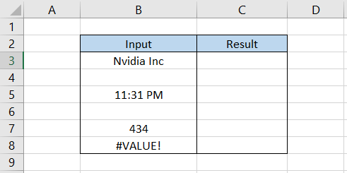
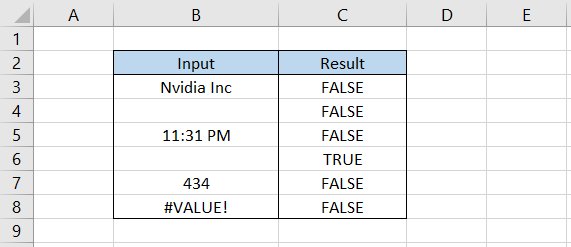
Let’s revisit the example. Suppose we have the data as illustrated below:
Here, we will use the formula =ISNONTEXT(B3) in cell C3 and drag it down till cell C8, which gives the result:
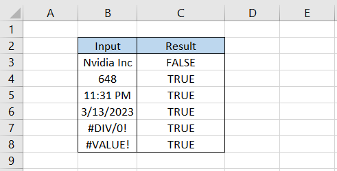
As we mentioned, all the results are reversed, i.e., text strings will evaluate FALSE while other data types will evaluate TRUE.
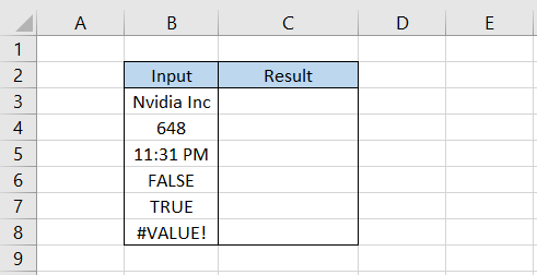
ISLOGICAL
ISLOGICAL is special because it evaluates to TRUE only when a boolean value is referenced in the function.
There are just two boolean values: TRUE and FALSE. If the function encounters either of those two values, it evaluates to TRUE or returns FALSE.
Below is an example of how the function works for different data types:
By using the formula =ISLOGICAL(B3) in cell C3 and dragging it down to cell C8, we get
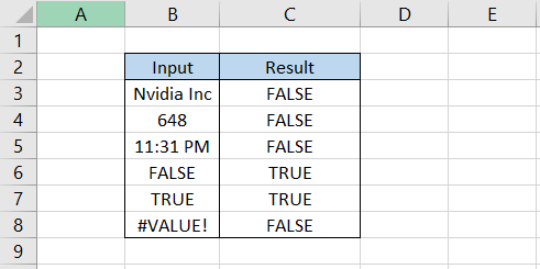
The function only returns the result as TRUE for boolean values TRUE and FALSE.
ISFORMULA
ISFORMULA, as the name suggests, will evaluate TRUE for all the referenced formulas.
For example, if you have the formula as =IF(1>0, “1 is greater than 0”, “1 is smaller than 0”), then the function will evaluate to TRUE despite the result being a text string.
However, it will also evaluate TRUE for the ISTEXT function since the result is ultimately a text string.
Similarly, all the numbers added in a cell using the equal sign will be considered a formula. So, for example, =987 will be 987 in the cell, yet it will evaluate to TRUE for both ISFORMULA and ISNUMBER functions.
Suppose we have the data as illustrated below:
By using the formula =ISFORMULA(B3) in cell C3 and dragging it down to cell C8, we get

Both values in cells B4 and B7 begin with an equal sign; hence, the result we get using the ISFORMULA function is equal to TRUE.
ISERROR
ISERROR is personally my favorite function for the lot. We now have the IFERROR function for error handling, but imagine what if the function did not exist?
In that case, most would have preferred to use the combination of ISERROR and IF functions. The former would have identified different errors, while the latter function would have returned the customized text strings.
Suppose we have the data as illustrated below:
Again, we use a similar formula =ISERROR(B3) in cell C3 and drag it down till cell C8, which gives the result:
The function works wonderfully for all types of errors, such as #VALUE!, #DIV/0!, #VALUE!, #REF!, #NUM!, and #NA! Etc.
If your objective is to identify only the ‘not available’ or the #NA! Errors, then you should use the ISNA function.
ISNUMBER
Aren’t these functions a bit too obvious? I mean, just look at the names! You might have already guessed that this one will evaluate the numbers, and you are absolutely right.
Let’s say we have the data as illustrated below:
Here, an important thing to remember is that even date and time values are stored as numbers in Excel. So don’t be surprised if you find that the function evaluates those as TRUE.
The formula will be =ISNUMBER(B3), which gives the result as
As stated earlier, even the time value returns the result as TRUE and the number in cell B7.
ISBLANK
Finally, we are at the final information function discussed in this article.
This one lets you easily identify all the blank cells in a given dataset without going through individual cells.
If you have read our articles on CHAR and CODE functions, you might remember that certain characters are not visible in the cell, yet they may exist in the spreadsheet.
The ISBLANK function and any other spreadsheet cell can easily identify such cells.
Suppose we have the data as illustrated below:
In this example, we see two different blank cells. After using the formula =ISBLANK(B3) in cell C3 and dragging it down to cell C8, we get
Since we have a non-printable character in cell B4, the function returns the result as FALSE, signifying that some type of character exists in the cell. Conversely, cell B6 is empty, so the function returns the result as TRUE.
And that is almost everything about the information functions!

Free Resources
To continue learning and advancing your career, check out these additional helpful WSO resources:


or Want to Sign up with your social account?