Equilibrium Quantity
It is the state of equilibrium in the market, where the quantity of a specific commodity aligns precisely with the consumer demand


What is Equilibrium Quantity?
Equilibrium quantity signifies the quantity of a good supplied in the market when the quantity supplied by sellers corresponds to the quantity demanded by buyers. This concept falls within the domain of market equilibrium and is interconnected with the notion of equilibrium price.
The market has achieved an ideal balance when prices have settled to accommodate the needs of all involved parties. Microeconomic principles provide a model to determine a product or service's optimal quantity and price.
It is based on the supply and demand model, which is the core principle of market capitalism. This theory assumes that producers and consumers exhibit consistent, predictable behaviors not influenced by external factors in their decision-making.
It holds a crucial position in determining the prices of products or services within a market because, with this equilibrium, an oversupply or undersupply could result in price instability.
Understanding the equilibrium quantity is essential for businesses as it enables them to foresee market dynamics, empowering informed decision-making and strategic planning.
- Equilibrium quantity refers to the state of equilibrium in the market, where the quantity of a specific commodity aligns precisely with the consumer demand, creating a balance state.
- The concepts of equilibrium quantity and price are fundamental elements in the broader microeconomic framework encompassing theories related to supply and demand, free markets, and capitalism.
- The supply and demand curves follow opposing paths and eventually cross, establishing economic balance and a corresponding equilibrium quantity.
- Various factors, such as consumer demand, product supply, pricing, and competition, all play a role in determining the equilibrium quantity. Any changes in these elements can cause a shift in the equilibrium quantity, either increasing or decreasing.
Understanding Equilibrium Quantity
Capitalism asserts that in a free market, supply and demand will naturally interact to create market efficiency and optimal pricing.
This means that an increase in demand relative to available supply usually results in higher prices, while an excess of supply compared to current demand tends to push prices lower.
The market naturally tends to find a point of equilibrium where the quantity of goods provided by producers matches the amount demanded by consumers.
The intersection of supply and demand determines the equilibrium quantity and price, where neither consumers nor suppliers have an advantage or disadvantage. This equilibrium price is viewed as the optimal price level.
Here, we see two distinct curves: one represents the supply of a particular product, while the other represents consumer demand.
These curves indicate the pricing (depicted on the vertical axis) and the quantity (shown on the horizontal axis) of the product.
The supply line exhibits an upward incline when observing from left to right. This is because price and supply share a direct correlation. A producer finds it more appealing to supply a good when the price is higher.
As the price of a product increases, so does the quantity supplied. In contrast, the demand curve, representing buyers, slopes downward. This decline occurs because there is an opposite relationship between price and the quantity that consumers desire.
Consumers are more inclined to purchase goods when they are inexpensive; hence, as the price of a product increases, so does the quantity supplied.
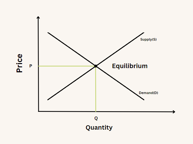
As the supply and demand curves follow opposite trajectories, they will eventually meet on the chart. This meeting point defines the economic equilibrium, representing the equilibrium quantity and price for a given good or service.
When the supply and demand curves intersect, and producers and consumers agree to produce or buy the equilibrium quantity of a good or service at the equilibrium price, it represents an ideal and efficient state for the market.
In theory, this is the natural equilibrium point towards which the market naturally tends.
Equilibrium Quantity Formula
The formula for equilibrium quantity is obtained by solving the linear equations formed by the supply and demand curves.
Let's take a basic linear supply function as an example:
y = mx + b
Where:
- x is the independent variable
- y is the dependent variable
- m is the slope
- b is the y-intercept (the line crosses the y-axis at this point)
Based on this linear function, the demand and supply equations are:
Qd = a – bP
Where:
- Qd is the quantity demanded
- P is the price of each unit.
- a represents the intercept term in the demand equation. It is the quantity demanded when the price is zero.
- b represents the slope of the demand curve. It reflects how much the quantity demanded (Qd) changes in response to a one-unit change in price.
Qs = x + yP
Where:
- Qs is the quantity supplied.
- P is the price of each unit.
- x is the intercept term in the supply equation. It represents the quantity supplied when the price (P) is zero.
- y is the coefficient associated with the price (P) in the supply equation. It represents the slope of the supply curve and reflects how much the quantity supplied (Qs) changes in response to a one-unit change in price.
At equilibrium, quantity demanded equals quantity supplied:
Qs = Qd
Substituting the respective formulas for Qs and Qd, we get:
x + yP = a – bP
Solving this equation provides the value of P, and substituting this value back into either the QD or Qs equation gives us the equilibrium quantity.
Example of Equilibrium Quantity
Let's consider the following example to understand how equilibrium quantity is obtained:
Example 1
Suppose the equation gives the demand for a product A:
Qd = 20 - P
Where Qd is the amount of product A that consumers want to buy (i.e., quantity demanded), P is the price of product A, and 20 is the intercept term or the quantity demanded when the price (P) is zero.
The supply of the same product is given by:
Qs = 5+2P
Where Qs is the amount of product A producers will supply (i.e., quantity supplied), 5 is the intercept term or the quantity supplied when the price (P) is zero, and 2 (the coefficient in front of P) indicates that for each unit increase in price, the quantity supplied increases by two.
Setting demand equal to supply:
Qd = Qs
20 - P = 2P + 5
Isolate the variable by adding P to both sides and subtracting 5.
20 - 5 = 2P + P
15 = 3P
Simplify the equation:
5 = P
The equilibrium price of product A is $5.
The equilibrium quantity can be found by plugging the equilibrium price into either the demand or supply equation.
The demand equation:
Qd = 20 - 5
Qd = 15
So, if the price is $5 each, consumers will demand 15 product units. Now, let's confirm the equilibrium quantity using the supply equation:
Qs = 2(5) + 5
Qs = 10 + 5
Qs = 15
Both the demand and supply quantities are equal to 15. This is an equilibrium quantity.
Example 2
Consider Company ABC, a popular store for smartphones. Every year, they usually buy 50,000 of these smartphones.
They observed that they often faced shortages towards the end of the year. Replenishing their stock becomes difficult during this time due to the increased demand for the product.
Due to this, they decided to buy 70,000 more smartphones and increase their prices. However, they had too much inventory by the year's end, indicating an overstock problem.
Following an in-depth market analysis, ABC adjusted its strategy. In the subsequent fiscal year, they scaled down their inventory to 60,000 units and offered a more competitive retail price.
This strategic shift resulted in successfully selling all units, pointing to an equilibrium quantity of 60,000 units for this smartphone model. This equilibrium strikes the perfect balance between supply and demand, effectively avoiding both stockouts and excess inventory.
Surpluses and Shortages
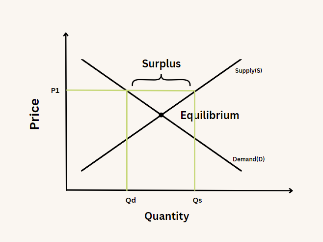
To understand the movement towards equilibrium of both price and quantity, let's explore the impact when the price differs from the equilibrium level, either exceeding or falling below it.
When the price surpasses the equilibrium level, sellers aim to produce more goods than consumers will buy, leading to a surplus.
In such a situation, sellers reduce prices to attract more buyers, causing the market price to decline until supply and demand quantities balance gradually.
When the price falls below the equilibrium point, sellers cannot supply as much quantity as consumers demand. This results in a market shortage, with excess demand, and some potential buyers may need help to purchase.
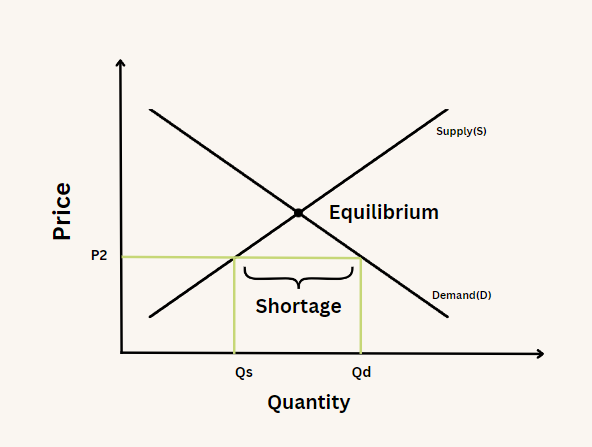
When this happens, eager buyers offer to purchase the product at a price surpassing the one initially set by sellers, causing the market price to go up gradually. Thus, quantities supplied and demanded move towards each other until they achieve equilibrium.
In both scenarios, the market naturally adjusts to achieve balance. Once equilibrium is reached, the established price and quantity remain unchanged unless an external factor causes a shift in the entire supply or demand curve.
Shifts in Demand and Supply
Shifts in supply and demand curves can be classified into four scenarios:
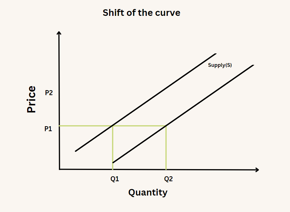
- The supply curve moves to the right when supply increases
- The supply curve moves to the left when supply decreases
- The demand curve moves to the right when demand increases
- The demand curve moves to the left when demand decreases
Shifts in Demand and Supply vs Movement
Distinguishing between shifts in the supply or demand curve and movements along the curve is important.
1. Curve Shift
A curve shift is indicative of a significant and widespread change in either the supply or demand for a product, impacting the entire curve across different price levels. These shifts are often prompted by fundamental alterations in various factors.
For instance, in the case of a demand shift, changes in consumer preferences, shifts in income levels, or sudden cultural trends can lead to an increase or decrease in demand.
On the supply side, shifts may arise from changes in production technology, availability of resources, government policies, or external shocks affecting the cost of production.
The direction of these shifts provides essential insights into market dynamics. An increase in demand, for example, results in a rightward shift of the demand curve, indicating a higher quantity demanded at all price levels.
Conversely, a decrease in demand shifts the curve leftward, suggesting a reduction in the quantity demanded at all prices. The same principles apply to supply, where an increase shifts the curve to the right, and a decrease shifts it to the left, affecting the quantity supplied at every price point.
To illustrate, consider a sudden trend in the fashion industry that makes a particular style highly popular. This surge in demand for trendy clothing leads to a rightward shift in the demand curve. Consequently, clothing producers experience increased demand at every price point, allowing them to adjust prices in response to the heightened demand, ultimately affecting market equilibrium.
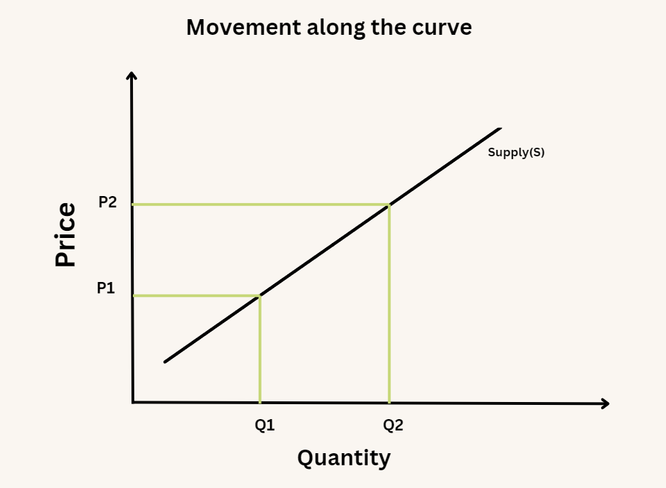
2. Movement along the Curve
Movements along the demand and supply curves, on the other hand, are specific to changes in the price of the product, while other factors remain constant. These movements represent variations in the quantity demanded or supplied in response to price changes.
For example, if the price of the trendy clothing mentioned earlier increases, leading to a decrease in the quantity demanded while other factors such as consumer preferences and income levels remain unchanged, this would be a movement along the demand curve.
In this scenario, consumers' purchasing behavior is influenced primarily by the change in price, without broader factors affecting demand undergoing a shift. Such movements provide valuable insights into how changes in price impact the quantity demanded or supplied within existing market dynamics.
Equilibrium and Economic Efficiency
Maintaining equilibrium is crucial for establishing a market that is both stable and effective. The competitive dynamics of that market ensure that resources are allocated optimally and reflect consumers' true value placed on goods and services.
Suppose a market is at its equilibrium price and quantity. In that case, it remains stable since it effectively balances the quantity supplied with the quantity demanded, which prevents any need for deviation from that point.
However, if the market is not in equilibrium, economic forces come into play to restore balance by adjusting the price or quantity. This adjustment occurs in response to imbalances, where there is either an excess of supply relative to demand or vice versa.
This equilibrium-seeking process is an inherent aspect of a free-market economy.
The equilibrium in a competitive market signifies efficiency, defined by economists as a state where improving one party's situation is impossible without imposing costs on another. Conversely, inefficiency arises when it becomes possible to benefit one party without imposing costs on others.
Market Dynamics and Limitations
The theory of supply and demand is a fundamental basis for economic analysis, yet economists advise against strictly interpreting it.
While a supply and demand graph illustrates, in isolation, the market dynamics for a particular good or service, real-world decision-making is influenced by numerous additional factors.
These include logistical constraints, purchasing power, and the impact of technological advancements or shifts in the industry, highlighting the complexity beyond the simplicity of a supply and demand model.
The concept needs to consider possible externalities leading to market failure.
The Irish potato famine in the mid-1800s is a great example of the limitation of this theory when Irish potatoes were sent to England despite the crisis.
Although the potato market seemed balanced, with Irish producers and English consumers content with prices and quantities, the devastating impact on the Irish population was overlooked.
Social welfare measures aimed at correction or government subsidies provided to support a particular industry can also influence the balance between the price and quantity of a product or service.
Equilibrium Quantity FAQs
Equilibrium quantity is the point where the quantity demanded by consumers equals the quantity supplied by sellers.
Determining the equilibrium quantity involves solving the demand and supply equation (Qa – bP = x + yP). After obtaining the equilibrium price, it can be plugged into either the demand or supply function to compute the equilibrium quantity.
Changes in factors such as consumer preferences, technology, input prices, or government regulations can shift demand or supply curves, affecting the equilibrium quantity.
When the market is not in equilibrium, there is either a surplus or a shortage of the product. A surplus occurs when the quantity supplied exceeds the quantity demanded, and a shortage occurs when the quantity demanded exceeds the quantity supplied.


or Want to Sign up with your social account?