LOOKUP Function
Returns a particular value from a referenced range of cells


What is the LOOKUP Function in Excel?
The LOOKUP function in Excel returns a particular value from a referenced range of cells.
One of the most common lookup functions everyone knows about is the VLOOKUP function. Apart from that, we also have the HLOOKUP, INDEX MATCH formula, and the newest XLOOKUP function.
You must be wondering - how is VLOOKUP different from the LOOKUP function?
The most significant difference would be that the LOOKUP function easily lets you search for a particular text string or a number in a row or column and return corresponding data from either the left or right side of the lookup column.
On the other hand, VLOOKUP works similarly; however, it is restricted to returning values only from left to right orientation.
This article will guide you on the LOOKUP function and how to use it, along with a couple of examples.
- LOOKUP searches a row or column for a lookup value and returns a corresponding result from left/right or above/below.
- It differs from VLOOKUP which only searches vertically and returns results horizontally.
- The lookup vector must be sorted in ascending order to avoid errors.
- LOOKUP can also find the last non-empty cell in a column or return the latest matching value.
- With newer functions like VLOOKUP and XLOOKUP, LOOKUP is less commonly used but can still be handy in certain lookup situations.
How to use the LOOKUP Function in Excel?
The LOOKUP is categorized under the Lookup & Reference function, which looks for a value from one row, a one-column range, or a particular referenced range.
The function basically looks for a value in a row or column and either returns the same value if it exists or has the ability to return another value from the corresponding row or column.
Formula (Vector)
The function has two different syntaxes, as illustrated below.
=LOOKUP(lookup_value, lookup_vector, [result_vector])
where,
- lookup_value = (required) the value which we intend to search
- lookup_vector = (required) one row or one column in which the lookup_value will be searched
- result_vector = (optional) the corresponding one-row or one-column from which the value will be returned
Note
If the result_vector argument is ignored, the function returns the lookup_value present in the lookup_vector. Excel will return an error to the user if no matches are found.
Another important thing to note is that lookup_vector should be in ascending order, or you will get misleading results.
Formula (Array) LOOKUP Function
The other is:
=LOOKUP(lookup_value, array)
where,
- lookup_value = (required) the value which we intend to search
- array = (required) range of cells consisting of different types of data, which will be evaluated for lookup_value
In the next section, we will see some examples and how to use the function.
LOOKUP Function Example
If you know how to use the VLOOKUP or the INDEX MATCH combination, using the LOOKUP becomes a lot easier. So you could say, in some way, LOOKUP is the precursor function for VLOOKUP.
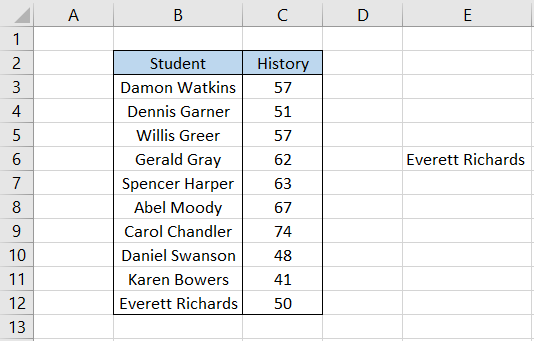
Suppose we have the data for the test scores as illustrated below:
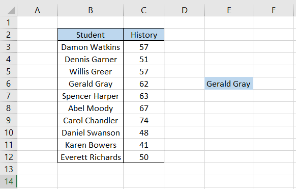
We need to determine the test score for Gerald Gray in History. First, we will return the students’ names in ascending order and their test scores in history. To do so, select the data and click Home > Sort & Filter > Sort A to Z.
This will give you the result:
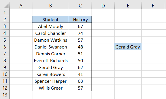
Next, all you need to do is use the formula =LOOKUP(E6,B3:B12,C3:C12) in cell E6, which gives the result:
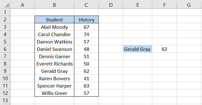
Thus, if we see our dataset, we will find that Gerald Gray scored 62 on his test.
Did you see what troubles we had to go through, though?
Firstly, we had to arrange the data in ascending order, and only we could find the exact result for the mentioned student.
Well, what if the data was not sorted in ascending order? Would the result vary, or would it be the same?
Again, we will use the same formula =LOOKUP(E6,B3:B12,C3:C12) on the unsorted data, which gives a rather contrasting result:
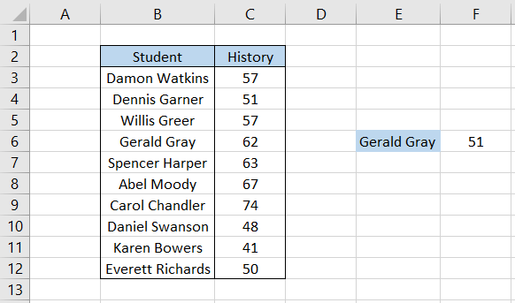
Gerald, my boy, did not score 51 on his test scores! It was Dennis who had a lower score. So you see the problem, unless you sort the data in ascending order and then use the LOOKUP function, you will get a contrasting result.
HLOOKUP Function
What if the data was rearranged in a horizontal orientation? Would the LOOKUP function still work?
Suppose we have the revenue numbers for a company in the horizontal orientation as illustrated below:
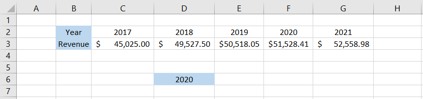
To get the revenue for 2020, we will just use the formula =LOOKUP(D6,B2:G2,B3:G3) in cell D6, which gives the result as
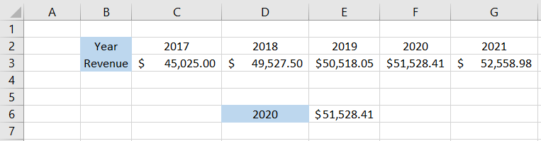
Thus, as you can see, we get the revenue number for 2020 quite easily, equaling $51,528.41. Since the data was already in ascending order, we did not get any deviating results.
What if the data was not arranged in ascending order?
In that case, we would have to arrange it in ascending order by transforming the data into vertical orientation and then again pasting the transformed data into horizontal orientation.
That’s quite a hassle, but it's one of the easiest methods you can follow to use LOOKUP on any type of data!

Uses of the HLOOKUP Function in Excel
Whether you're organizing a database, managing large volumes of data, or performing intricate calculations, the HLOOKUP function can provide efficiency and accuracy.
Let's explore some of the uses of this versatile function to help you streamline your tasks and boost your proficiency in Excel.
1. Finding the last non-empty cell
Apart from the basic function of looking up a particular value in the dataset, the function can also be used to find the last non-empty cell in a given dataset.
Suppose we have the data in the spreadsheet as illustrated below:
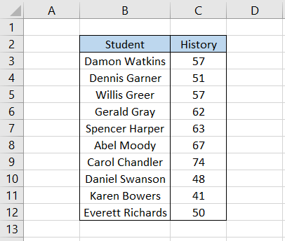
Here, we will use the formula =LOOKUP(2,1/(B:B<>""),B:B) in cell E6, which gives the last cell value as ‘Everett Richards’ in column B.
Well, what if we had a couple of blank cells in column B? Would the formula still work?
Suppose the data looks as illustrated below:
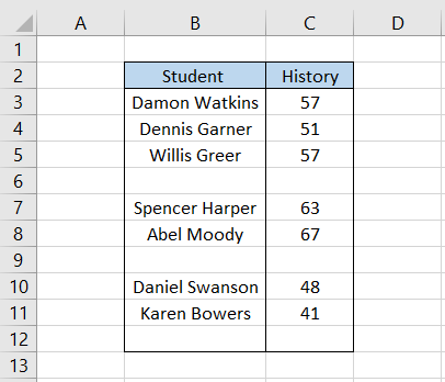
Again, we will use the formula =LOOKUP(2,1/(B:B<>""),B:B) in cell E6. So you see, despite having a couple of blank cells in our dataset, the formula still captured that ‘Karen Bowers’ was the last non-empty cell in column B.
Note
The formula only evaluates the column referenced in the formula. For this example, the referenced range was B:B; hence, the presence or absence of values in column C won’t affect the final result.
2. Returning the latest values
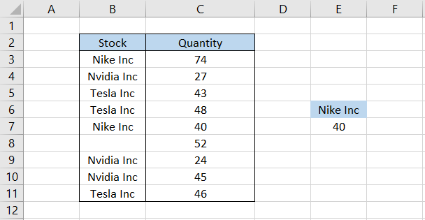
Suppose that you are a day trader and make a series of trades in a couple of stocks as illustrated below:

You need to know how many quantities of stocks were traded in the last ‘Nike Inc’ order. For this, we will use the formula =LOOKUP(2,1/(B3:B11=E6),C3:C11) in cell E7, which gives the result:
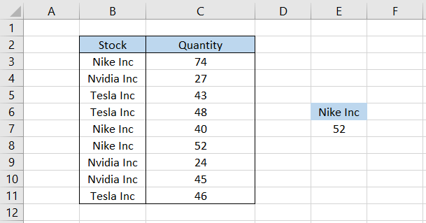
The function evaluates two ranges, i.e., B3:B11, where it checks for the text string ‘Nike Inc,’ the cell value in E6. Another range compared is C3:C11, which gives the corresponding quantity of stocks traded.
If we delete the latest value from column C, the formula returns the result as zero since the cell is empty, as illustrated below:
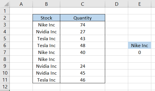
However, when we delete the text string from column B and instead keep the number, the function will look for the next latest number, which is in cell C7.
The LOOKUP function may not look much, but it is quite handy once you get used to it. But considering the presence of VLOOKUP, INDEX MATCH, and the very recent XMATCH, we believe you might hardly get a chance to try it!


or Want to Sign up with your social account?