Quantity Theory of Money

What Is the Quantity Theory of Money?

The quantity theory of money states that an economy's price level and money supply are directly proportional. Therefore, money supply changes correlate with price changes and vice versa.

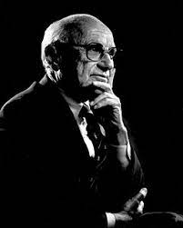
This theory was introduced by a Polish mathematician named Nicolaus Copernicus in the year 1517 and was later popularized by the economists Milton Friedman and Anna Schwartz.

Economists, including Simon Newcomb, Alfred de Foville, Irving Fisher, and Ludwig von Mises, improvised and modified the quantity theory with time.

Reviewing the actions of the Federal Reserve or European Central Bank (ECB) reveals that if this organization increases the economy's money supply by twice the usual amount, commodity prices will likely rise rapidly in the long run. 

The surplus money supply might be linked to this price increase because it will raise demand and spending.

This change results in consumers paying twice as much for the same amount of goods and services. As a result, inflation levels tend to increase. 

However, academics disagree that prices would shoot up with a change in the amount of money in circulation.

A framework for understanding how price changes impact the supply or circulation of money in an economy is said to exist in the quantity theory of money.

The Classical Quantity Theory of Money

The principle of classical theory is based on an automated economy. Therefore, the economy always has the potential to achieve the natural level of real GDP or output. 

The natural level of GDP is the level of GDP in a given year when there is no tendency for the inflation rate to either accelerate or decelerate. The actual GDP level is reached when the economy's resources are utilized fully.

The Classical Quantity Theory is often expressed using the equation of exchange,

MV = PQ

where

• M = money supply
• V = velocity of money
• P = price level
• Q = quantity of goods and services exchanged

This equation asserts that the total amount of money spent in an economy (MV) must equal the total value of goods and services produced and sold (PQ).

Assumptions

The two key assumptions are:

1. Full Employment: The Classical Quantity Theory makes the long-term assumption that the economy runs at full employment. This suggests that rather than having an impact on output or employment levels, changes in the money supply essentially affect pricing.
2. Flexibility of Prices: The idea that wages and prices are fluid and swiftly adapt to shifts in the money supply is another fundamental premise. According to this theory, every increase in the money supply will cause prices to rise without having an impact on actual economic factors.

Criticism

The criticism and limitations of the theory are:

1. Money's Velocity Is Not Constant: According to critics, the notion that money moves at a constant pace is impractical since it might vary over time as a result of modifications in consumer behavior, financial innovation, or changes in the state of the economy.
2. Short-Run Dynamics: While sticky prices and wages can have an impact on how monetary policy is transmitted to the actual economy, the Classical Quantity Theory ignores these dynamics in favor of long-run linkages between money and prices.
3. Demand for Money: The idea fails to take into account the influence of the demand for money, which varies depending on variables like interest rates, level of certainty, and liquidity preferences. Shifts in the demand for money can affect monetary policy's ability to impact economic outcomes.

Fisher's Quantity Theory of Money

Price levels increase in direct proportion to decreased values of money, and vice versa, which is the essence of Fisher's Quantity Theory of Money.

Demand and supply of money also determine the value of money or the price level.

An equation explaining Fisher's theory is :

MV = PT or P = MV/T

(M)(V)=(P)(T)

Where,

• M = Money Supply
• V = Velocity of circulation (the number of times money changes hands)
• P = Average Price Level
• T = Volume of transactions of goods and services

Example 

Let's analyze Fisher's quantity theory of money with the help of an example. Assuming M = $500. M’ =$100, V = 5, V’ = 10, T = 350 goods.

We have

P = (MV+M’V’)/T

P = (500*5+100*10)/350

P = $10.

If the money supply is doubled, P = $20

Value of money = 1/20.

As a result, when the money supply is doubled, the value of money is reduced. Similarly, when the value of money is halved, P = 5$, and the value of money = 1/5, which is twice the initial value.

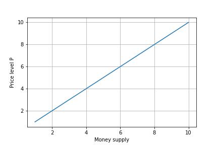
The graph above shows the linear relationship between money supply and price. 

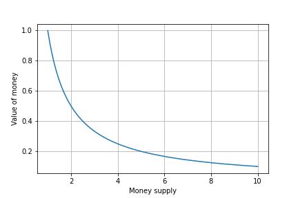
The money supply vs. value of money graph is hyperbolic, which shows an inverse relationship between the two.

Assumptions 

Fisher's theory is based on the following assumptions:

1. Constant Velocity of Money: Fisher assumes an idealistic approach to the velocity of money that remains unaffected by factors such as population, interest rates, and economic situations that affect the velocity of money in realistic conditions.
2. Constant Volume of Trade or Transactions: Fisher assumes the total volume of trade (T) will remain constant regardless of the amount of money in circulation. To maintain constant T, it is a must to employ all resources in the economy, which is not possible.
3. Price Level is a Passive Factor: Fisher's equation's price level (P) is a passive factor. This means that it affects the other aspects of the equation but doesn't affect them directly.
4. Money is a Medium of Exchange: Money is assumed to facilitate exchange rather than serving as an asset. 
5. Constant Relation between M and M': Commercial banks obtain bank money by creating credit, a function of currency money (M). As a result, the M' to M ratio remains unchanged, and adding M' to the formula does not change the quantitative relationship between M and P.
6. Long Period: Fisher's theory requires the assumption that V and T remain constant over a long time. 

Criticism and limitations

It is considered an obvious fact rather than a theory. It does not show the cause and the effect clearly. It simply shows what has happened. The theory assumes that other things like V, V', M', and T remain constant, which is unreal.

It isn't possible to explain the trade cycle with the transactions approach to the quantity theory of money, although it may suffice in explaining long-term price trends.

The theory was challenged by Cambridge professors, who came up with a new approach. The critics suggest that in the short run, prices are sticky, so the direct connection between money supply and price level no longer holds.

Cambridge's quantity theory of money

In contrast to Fisher's emphasis on using money as a medium of exchange, Cambridge's theory emphasizes money as an asset.

The money exchange function eliminates the problem faced by the barter system of a double coincidence of wants.

A. Marshall's Equations

M = KY + KA

Here

• M = Total money in circulation and deposits with the bank
• Y = Total monetary annual income.
• K = The part of the income that people keep in liquid form for future use
• K' = The amount of property which is in the form of money
• A = The total value of the property

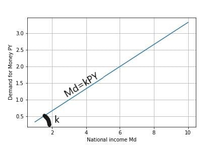
The amended form of this equation can be given as

M = KPY

• M = Supply of Money
• P = Price Level
• Y = Total Real Income
• K = The part of real income people want to keep in cash.

B. Prof. Pigou's equation

P = KR/M

• P = Common Price level
• M = Total amount of money
• R = Total real income of the society.
• K = The part of real income which is kept in the form of money

C. Robertson's Equation

M = PKT

Where M, P, K, and T are the same as the above equation

The demand for money depends on the liquidity preferences of the people. Most people who earn tend to save in the bank or invest in assets that cannot be sold instantly. This money invested cannot be called liquid cash.

Many factors influence the demand for money 

• The period of obtaining income
• Distribution of national income
• The velocity of circulation of money
• Population
• Trade cycle
• Banking habits

Cambridge's Quantity Theory of Money ideology is superior to Fisher's transaction ideology in the Quality Theory of Money.

Features of Cambridge's Theory

The main features of Cambridge's Theory 

1. A Part of Income is kept in the Liquid Form: Economists at Cambridge believe that nobody can predict the future. This assumption made them think that people tend to save for emergencies.
2. Completeness: Essentially, the value of money is determined through demand and supply, which is given priority in Cambridge's theory.
3. Liquidity Preference: In the Cambridge equation, emphasis is placed on Liquidity Preference. The basic tendency of saving is considered in Cambridge's theory. The basis of Keynes's 'Liquidity Preference Theory' is from here.
4. Related to Short-Term: While Prof. Fisher's equation only analyzes long-term changes, Cambridge's analysis also presents the solution to short-term changes.

Criticism

The critics have criticized this theory on the following bases:

1. Prof. Pigou's equation shows the demand for money for consumer goods, while in practical life, there is a demand for money for many reasons.
2. The demand for money has been considered the current deposits at banks. Therefore, it has been supposed that a current deposit with banks is a part of income. 
3. However, if a trader takes a bank loan and then deposits it as a current deposit, this is not considered a trader's income.
4. Fixed deposits in banks are not taken into consideration
5. The Cambridge equation does not specify how changes in income and savings will alter prices.
6. The increase in production and income can't be concluded based on this equation.
7. The size of the cash reserve has been hypothesized to be influenced by K when it is influenced both by R and K.
8. The Cambridge equation ignores speculative demand for money, but there is also demand for this
9. Keynesian economists and Milton Friedman further improvise these theories.

Fisher's equation only applies to economies with full employment, but the Cambridge equation is applicable in all circumstances.

Keynesian economists

John Maynard Keynes (1883–1946), considered the father of modern macroeconomics, gave Keynesian economics its name, theories, and principles.

Economics based on Keynesian principles emphasizes the importance of government intervention and activist stabilization policies to influence aggregate demand and improve economic prospects.

As Keynes noted, increases in the money supply led to a decrease in the velocity of money circulation while real income–the flow of money toward factors of production–increased.

According to Keynes, a high or excessive savings rate could adversely affect the economy by reducing the amount of money circulating in it.

Equation

While quantity theorists have considered the aggregate money supply largely exogenous, Keynesians have considered it largely endogenous and a function of the fundamental factors determining production and trade.​

Aggregate demand according to Keynesian = C + I + G + NX

Where,

• C = Consumption (by consumers who buy goods and services)​
• I = Investment (by businesses to produce more goods and services)​
• G = Government spending
• S = Net exports (value of exports minus imports)

Keynesian theory was used in developing the Phillips curve, which examines unemployment and the ISLM Model.

These days, many governments use Keynesian theory portions to smooth out their economies' boom-and-bust cycles.

Criticisms

Friedman, the critic who shifted the focus of study from aggregate demand to the role of money supply in inflation, developed the monetarist school of thought (monetarism).

Critics of the Keynesian theory say that it favors centralized planning. If the government is expected to spend money to prevent depression, it is assumed to know what is best for the economy. The impact of market forces on decision-making is thus eliminated.

Friedman's Quantity Theory of Money

In his 1956 article, "The Quantity Theory of Money-A Restatement," Friedman reformulated the old quantity theory of money.

Rather than being a theory of output, income, or prices, Friedman's quantity theory is a theory of demand for money.

According to Friedman, money demand can be divided into two types.

1. In the first category, money is required for transactional purposes. It functions as a means of exchange. This perspective on money is similar to the traditional quantity theory.
2. On the other hand, money is demanded in the second category since it is regarded as an asset. 

Money, unlike a medium of commerce, has a higher inherent value. It is a temporary storehouse of purchasing power and an asset or a component of wealth.

Three factors influence the demand for money

1. Total wealth to be held in various forms, 
2. The price or rate of return from these multiple assets,
3. Management of assets by the asset holder

Friedman distinguishes five basic types of wealth: money (M), bonds (B), equities (E), non-human physical goods (G), and human capital (H).

Total wealth encompasses all forms of "revenue" in a broad sense. For example, Friedman uses "income" to refer to "total nominal earnings," which is the average projected return from assets over a lifetime.

Friedman's Demand Function

Friedman's demand function is based on the above assumptions and formulations.

Eq1

M=f[p,RB-1rb.debt;re+1p.dpdt-1redredt;1pdpdt;w;y;m]

Where,

• M = the aggregate demand for money
• P = the general price level, 
• RB = the market rate of return for bonds, 
• re in the market rate of return for stocks, 
• 1/p. DP / DT is the nominal return on physical goods, 
• W = the ratio of non-human wealth to human wealth, 
• Y = the monetary return to wealth holders, and
• m = the variable that affects the tastes and preferences of wealth holders. 

Assuming that RB and re are stable, Friedman replaces the equation's variables representing bond and stock returns.

Eq2

[rb, 1 rbdrbdt]+[re+1p.dpdt1rb.dredt]

Furthermore, Friedman says there will be a proportional change in demand when there are changes in price and money income. 

This means that Equation 2 must be considered first-order homogeneous in P and Y for Equation 2 to become 

Eq3

IM=f(P;RB;re;1P.dpdt .w;y;)

Taking =1/p

Eq 4

MP=f(RB;re.1P.dpdt;w.P;)

In this form, Equation 4 represents the need for an actual remainder as a function of the "real" variable." 

Dynamics of Monetary Policy and Economic Equilibrium

Friedman argues that money supply and demand are independent in his quantity theory of money.

Due to the actions of the monetary authorities, the money supply changes, while the need for cash remains more or less stable. This means that the amount people want in cash or bank deposits is more or less related to their permanent income. 

If the central bank buys securities, the people who sell the securities to the central bank receive the money, which increases their cash holdings. 

People will spend this excess money partly on consumables and property purchases. These expenditures will reduce their cash balances and, at the same time, increase the national income. 

On the other hand, when the central bank sells securities, people's money holdings fall below their regular income.

As a result, they will strive to boost their cash on one hand by cutting Consumption and, on the other hand, by selling assets. As a result, the demand for money remains constant in both circumstances.

If a monetary demand is made, the effect of changes in the money supply on expenditure and income can be predicted. 

If the economy is below full employment, the money supply will increase spending, output, and work. However, this is only possible in the short term. 

Graphical explanation of Friedman's quantity theory

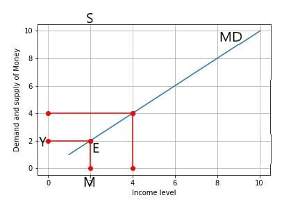
While the X-axis depicts money demand and supply, the Y-axis represents income level. MD is the money demand curve, which changes with income. MS is the money supply curve. 

The equilibrium income level OY is determined whenever these two curves converge at point E. Assume that the monetary base rises and the supply curve switches to M1S1.

At this point, the collection outstrips supply, creating a new equilibrium at E1. As a result, income increases to OY1 at the new equilibrium level.

Conclusion

The Quantity Theory of Money can provide important insights into the connection between the money supply, pricing, and economic activity.

Although it originated with classical economic theory, economists like Friedman have since deepened and broadened our grasp of it.

The theory provides a framework for examining the macroeconomic effects of changes in the money supply by taking into account the dynamics of money demand and the effects of monetary policy on spending and income.

Like any economic theory, it is not without flaws, though, especially when it comes to its presumptions about the stability of money demand and the predictability of its effects on the economy.

In macroeconomics, the Quantity Theory of Money continues to be a fundamental idea that guides conversations about monetary policy, inflation, and economic stability.

Free Resources

To continue learning and advancing your career, check out these additional helpful WSO resources:

• Balance of Payments
• Balance of Trade (BOT)
• International Monetary Fund (IMF)
• Quantitative Easing
• Quantitative Tightening