Capital Budgeting Best Practices
Standards or guidelines that are generally accepted and used in capital budgeting.


What is Capital Budgeting?
Capital budgeting refers to the systematic process of analyzing different projects under several cost and cash flow assumptions to determine which project is the most favorable to pursue.
Companies frequently use their cash flows for operating, investing, and financing. In the context of capital budgeting, this decision-making process pertains to investment activities.
If companies want to continue growing, they must invest in capital-intensive projects, such as property, plant, and equipment (PP&E) purchases, labor expansions, research, and development product undertakings, among others.
Analyzing independent projects is simple enough in the sense that management would evaluate different projects solely on their basis of profitability and pick the profitable ones.
Nonetheless, most decisions face budget constraints and thus must choose only one at a time; these types of projects are known as mutually exclusive projects.
Generally speaking, when evaluating several mutually exclusive projects at the same time, management ends up picking the project that generates the most economic value for the firm. Capital budgeting is about estimating such value in absolute and relative terms.
To have a solid understanding of how to perform a capital budgeting exercise, it’s imperative to understand the various investment criteria used in this decision-making process.
Once armed with these project criteria tools, the next step involves performing the actual calculations of the project's cash inflows and outflows. This process involves having several assumptions in mind since the evaluation of cash flows by themselves are not as intuitive as one may think.
A final consideration in capital budgeting involves performing a "what if" project analysis. Using sensitivity, scenario, and NPV break-even analysis will help determine a project's profitability under different detrimental or beneficial assumptions.
- One of the best practices in capital budgeting is to thoroughly evaluate potential projects by assessing expected cash flows, project costs, risks, and strategic alignment with the company’s long-term goals.
- Incorporating risk analysis into the capital budgeting process is crucial. This includes identifying potential risks associated with a project, such as market risks, operational risks, and financial risks.
- Engaging key stakeholders throughout the capital budgeting process ensures that all relevant perspectives are considered.
- Best practices in capital budgeting involve ongoing monitoring and review of projects. This includes comparing actual performance against initial projections and making necessary adjustments.
Investment Criteria Used For Capital Budgeting
To determine what makes a good investment rule, investment criteria should adjust for the risk and time value of money and must be able to measure the value created for a firm.
A project’s risk and time value of money are accounted for via the process of discounting at a rate equal to a company’s cost of capital (WAAC). On the other hand, value can be measured in several ways, but the most common method is called net present value (NPV) analysis.
Payback rule
The payback rule dictates that you accept a project based on the cash flow's payback period and a specified cutoff period. The payback period refers to the amount of time it is required for an investment to break even.
Example:
| Project | C0 | C1 | C2 | C3 | C4 |
|---|---|---|---|---|---|
| A | -2000 | 0 | 1000 | 1000 | 0 |
| B | -1000 | 0 | 1000 | 2000 | 3000 |
| C | -4000 | 1000 | 900 | 1000 | 2000 |
The payback period for Projects A, B, and C are 3, 2, and 3.55 years (by interpolation), respectively, assuming each cash flow (C0, C1,..., C5) is received at the end of the year. However, if you use a cutoff period of 3 years, projects A and B are the only ones you would accept.
One of the major disadvantages of the payback rule is that it does not consider cash flows after the payback period. The payback rule also ignores the time value of money (TVM), which means that it does not adjust cash flows for risk directly via discounting at an appropriate rate.
On the other hand, one must acknowledge that the payback rule has a systematic bias against large investments with longer paybacks and favors small investments with shorter paybacks.
As such, one must be careful of solely depending on this method despite its simplicity and intuitiveness.
Chances are that capital expenditures for long-term assets, such as PP&E or R&D, are necessary for a firm's long-term success. Therefore, the payback rule seems most appropriate for short-term projects. Long-term projects, on the other hand, should ideally be analyzed through a net present value (NPV) analysis.
Net present value (NPV)
The NPV analysis helps estimate the dollar value of a project’s cumulative cash flows today, net of initial cash outflow from undertaking the project. To calculate NPV, we must discount each project’s cash flows and subtract the initial cost.
NPV = C0 + C1 (1 + r)-1 + C2 (1 + r)-2 + ... + Cn (1 + r)-n
Cash inflows are entered as positive, while cash outflows are entered as negative. In theory, NPV is the best way to value cash flows than the payback rule since it properly accounts for the time value of money and cash flow riskiness via discounting.
NPV may sometimes be difficult to apply due to an inappropriate discount rate or cash flow estimates.
Example: Assuming the discount rate, r = 12%;
| Project | C0 | C1 | C2 |
|---|---|---|---|
| A | -800 | 1000 | 1000 |
- NPV = -800 + 1000 (1 + 0.12)-1 + 1000 (1 + 0.12)-2 = 890.05
- NPV = -800 + present value of a $1000, 2-year annuity at a 12% rate
= -800 + 1000 [{1 - (1 + 0.12)-2}/ 0.12] = -800 + 1,690.05 = 890.05
If the NPV of the project is greater than zero, you should accept the project as the investment is said to create value for the company.
A disadvantage of NPV analysis is that it doesn’t account for project size. For example, an NPV of $50 for a project that costs $50 is technically as good as a project that initially costs $500 and ends up with the same NPV of $50.
Nonetheless, NPV is theoretically appealing as it estimates the direct expected increase (decrease) in firm value and, thus, a proportional increase (decrease) in the company's stock price:
Example: Assume a company currently has 400 million common shares outstanding, and its current market price is $50. All things equal, what is the theoretical effect on the company’s stock price if the company invested in a $500 million project that yielded $800 million in after-tax discounted cash flows?
Answer: ABC’s stock price should increase by $0.75
New share price: 50 + (NPV per share) = 50 + {(-500m + 800m)/ 400m} = $50.75
In reality, though, all things are not equal. A company’s stock price fluctuates mostly due to the present value of future earning expectations.
An alternative yet financially sound way to see if a company is constantly creating value for its business is by looking at a company's return on invested capital (ROIC), return on total capital (ROTC), or operating return on assets ( operating ROA) and compare it against the company's weighted average return on capital (WACC).
Since a company's WACC captures a firm's average risk, a company with an ROIC greater than its WACC means that management actively increases shareholders' wealth via firm value creation. The opposite also holds with ROIC less than WACC.
For the purpose of this analysis, a company's ROIC, ROTC, and operating ROA are calculated as follows:
1. ROIC1 = after-tax net profit in a given period/ average book value of total capital in a given period
2. ROIC2= or net operating profits after tax/ average total capital = NOPAT/ average total capital * EBIT(1-tax)/ Average total capital
Note
Since ROIC1 is a measure of the return from all sources of capital (both equity and debt), after-tax interest expense (interest expense is tax deductible) needs to be added to the net income to capture all net income available to both sources; this is known as after-tax net profits.
Similarly, ROIC2 uses EBIT(1-tax) in the numerator can be achieved by subtracting after-tax non-operating income from after-tax net profits. This numerator is a measure of profits that assumes the company did not receive any tax benefits from holding debt.
The denominator for both versions of ROIC is the sum of the average book value of short-term debt, long-term debt, common equity, and preferred equity. By this definition, working capital liabilities are excluded from the calculation. An alternative in calculating total capital is to use average total assets altogether.
3. ROTC = EBIT/ average total capital
4. Operating ROA = operating income/ average total assets or EBIT/ average total assets

Internal rate of return (IRR)
The IRR is the percentage equivalent of NPV, defined as the discount rate that makes the NPV of a project equal to zero.
A correct IRR is one that allows the following relationship to hold:
Present value of outflows = Present value of inflows
Despite the difficulty in manually calculating the internal rate of return via a trial-and-error method, you can easily do it with a simple excel IRR function. All financial calculators also solve for IRR.
The IRR is more intuitive than the NPV because the rate of return essentially summarizes a project’s investment merits. Generally speaking, the IRR rule states that a project is accepted if the project's IRR exceeds the weighted average cost of capital (WACC).
IRR decision rules:
- If IRR = WACC, NPV = 0
- If IRR > WACC, accept the project because NPV > 0
- If IRR < WACCC, reject the project because NPV < 0
Under this context, the minimum IRR needed to accept a project is commonly known as the hurdle rate. Projects with IRRs greater than this rate will be accepted. The opposite is true with projects that carry lower-than-hurdle-rate IRRs.
IRR can be further thought of as the expected return on an annual basis, which makes much more intuitive sense. Moreover, the IRR tends to provide the same project decision as the NPV rule as long as it falls smoothly as the discount rate increases:

As mentioned numerous times, the biggest advantage of the IRR is its intuitive appeal and ability to summarize an investment's merits. IRR shows a project's profitability in percentage terms or the return on each dollar invested.
Similarly, if a project's IRR is big enough, say 50%, then there is no need to calculate the WACC to calculate NPV. Also, IRR provides information about a project's margin of safety, unlike NPV; it lets you know how much a project's return can fall before turning negative.
A project is said to generate conventional cash flows if the sign of these cash flows changes. On the other hand, unconventional cash flows have more than one significant change, which may be problematic for analytical purposes.
Projects that are expected to produce uneven cash flows will produce multiple IRRs. The final potential problem is that using IRR can lead to an incorrect decision if you are analyzing two mutually exclusive projects.
Furthermore, IRR also does not account for project size since IRR simply compares cash flows to the initial outlay (i.e., it does not capture the magnitude of the cash flows and thus profits).
If two projects cant happen at the same time and thus you can just pick one of them, then picking the project with the highest NPV is advised.
IRR assumes reinvestment at the IRR rate, whereas NPV assumes reinvestment at the cost of capital. IRR mathematically assumes a more aggressive reinvestment rate than NPV.
Note
Do not confuse IRR with cross-over IRR. The cross-over IRR provides the IRR that causes both projects to have the same NPV (NPV intersection).
Example: Imagine you are comparing two projects, A and B. Assume project A is preferable when your discount rate is 15% but no more than 23.22%. In contrast, project B is preferred whenever your cost of capital increases above 23.22%. In this case, your cross-over IRR is 23.22%.
Profitability index (PI)
PI is defined as the present value of an investment's future cash flows divided by the investment's initial cost. Hence, this ratio measures the dollar value created per dollar invested.
This method is very useful when dealing with a tight budget. In other words, whenever a company has scarce amounts of capital available to invest, the profitability index is a useful tool to help allocate funds most efficiently; a project in which each dollar invested yields the greatest value created (in comparison to other mutually exclusive projects)
PI = present value of future cash flows/ initial outlay = C1(1 + r)-1 + C2(1 + r)-2 + ... + Cn(1 + r)-n/ c0
The general rule under this scenario is to accept the project with the highest PI first. However, if a project or group of projects carry a higher combined NPV, the latter should be accepted.
Example:
| Project | C0 | C1 | C2 | PV | PI | NPV |
|---|---|---|---|---|---|---|
| A | -10 | 30 | 5 | 33.1 | 3.31 | 23.0 |
| B | -5 | 5 | 5 | 22.9 | 4.58 | 17.9 |
| C | -5 | 5 | 15 | 18.4 | 3.67 | 13.4 |
Assuming a discount rate of 5%, if a company has three investments to pick from but under the condition that it can only spend $10, then project B and C should be taken since their combined NPV are greater than Project A alone, despite having lower individual profitability indexes.
Making capital investment decisions
This section is about analyzing different types of cash flow projects and, most importantly, determining what information is relevant for analysis.
Types of capital allocation project
Common project proposals include:
- Replacement projects to maintain existent business operations
- Purchase or replacement of new property plant and equipment (PP&E)
- Expansion projects
- Launching new products or developing a new market
- Mandatory projects required by government agencies or an insurance company
- Pollution control devices
- Other environmental or safety-related projects
- These types of projects are not expected to generate revenue as their main drive is compliance. Mandatory projects, however, tend to be required or parallel to other revenue-generating projects.
- Other projects:
- Research and development (R&D)
- These types of projects, along with investments in new PP&E, could be labeled as cost-reduction projects if their purpose involves reducing costs via increased operational efficiency.
- Exploration
- Management pet projects
- Research and development (R&D)
Where projects 3 and 4 are aimed at increasing sales, whereas project 2 is aimed at cost reduction. Furthermore, replacement projects are very frequent and don't require detailed analysis.
On the other hand, replacement projects need a fairly detailed analysis of the matter to determine the equipment’s average total life, average age, and remaining life. Similarly, expansion projects need careful forecasts of future demand.
The same detail is also needed in projects aiming to create needed products or develop a new market for their products. Given the vast uncertainty involved in this type of project, careful detail analysis is certainly a must.
The capital allocation process: key principles
When evaluating projects, there are roughly 10 important assumptions to consider.
Many analysts make the mistake of not including all of these, so careful consideration of all of these assumptions will help you forecast cash flows and reach a project decision that is both well-structured and accurate.
For the purpose of this discussion, it is important to point out that capital budgeting is as good as the assumptions you input into the model, just like any other financial model. Nonetheless, your project evaluation should be deemed trustworthy by ensuring your assumptions are disciplined and well-rounded.
The ten assumptions below should help you get started:
Step - 1: Evaluate the Project based on Incremental Cash Flows, not Accounting for Income/Profits
Incremental cash flow refers to the additional change in cash flows created from undertaking a project, not the full amount. This concept is known as the stand-alone principle. Similarly, only those cash flows that directly result from undertaking a project should be included.
Hence, only incremental cash flows resulting from undertaking a project should be considered in the capital allocation process.
NPV analysis commonly analyzes operating cash flows, not profits. The main difference between cash flows and profits is that profits take into account depreciation expenses.
Also, unlike cash flows, sales and expenses for the purpose of calculating profits are reported based on accrual accounting and the matching principle.
Under accounting rules, when a company makes an expenditure, it may either capitalize the cost as an asset or expend it. However, if the expenditure is expected to provide future economic benefits over many accounting periods, then the expense is capitalized.
Whenever an expense is capitalized, such as in the case of replacing PP&E, the expense is initially recorded on the balance sheet at its cost (fair value plus any costs necessary for readying the asset).
As time goes by, the expense is allocated to the income statement as depreciation expense over the life of the (tangible) asset. Amortization would be calculated if the expense involved an intangible asset acquisition.
When using profits, depreciation defers expenses as it evens them throughout the asset’s useful life (assuming the straight-line method).
Despite these accounting differences, for NPV calculation purposes, cash flows are used when they occur.
WSO Pro Tip
If you are unaware or just rusty with your accounting skills, don't worry! WSO provides a comprehensive guide on accounting foundations for beginners.

Example 1
Company ABC is considering the purchase of a piece of equipment to fulfill the demand for its textile products effectively.
The total cost of the equipment, including transportation and other additional costs to ready-to-operate the asset, would be $98K. ABC’s management also estimates that the net operating cash flows would be $21.5K annually. The equipment is expected to have a useful life of 20 years.
The equipment’s salvage value is $5K; hence, assuming a straight-line depreciation, the annual depreciation is $4,650 per year ((98K-5K)/20). ABC does not pay taxes as the company is registered as a not-for-profit firm. Furthermore, ABC’s management determined that their project-specific WACC is 12%.
NPV using cash flows:
NPV = Initial Cost + PV of Future Cash Flows
NPV = initial cost + PV of a 21.5K annuity for 20 years at a 12% discount rate + PV of salvage value
NPV= -98K + 21.5K * {1 - (1 + 0.12)-20/ 0.12} + 5K * (1 + 0.12)-20
NPV = $63,111.37
NPV using profits:
NPV = PV of profits
NPV = PV of operating profits less depreciation expense
Note: each year, the equipment is expected to produce profits of ($21.5K - $4.65K) and $16.85K
NPV = PV of a 16.85K annuity for 20 years at a 12% discount rate
NPV = 16,850 * {1 + (1 + 0.12)-20/ 0.12} = $125,860.13
Notice how in NPV using profits, the initial cost of equipment is not expensed but rather capitalized and thus expensed via depreciation expense over the course of the asset's useful life.
This process of cost deferral artificially inflates the NPV of the project compared to an NPV analysis using operating cash flows.
Similarly, the timing of other cash flows, such as in accounts receivables and accounts payables, also causes profits to differ from cash flows.
For instance, if ABC had postponed the initial cost by one year, then NPV using profits would remain uncharted. This isn't the case for cashflows:
NPV = PV of initial cost + PV of a 21.5K annuity for 20 years, at a 12% discount rate + PV of salvage value
NPV = -98K * (1 + 0.12)-1 + 21.5K * {1 - (1 + 0.12)-20/ 0.12} + 5K * (1 + 0.12)-20
NPV = $76,611.37
As seen, NPV using operating cash flows increases by more than $10K only by deferring the initial cost by 1 year.
2. Time value of money
A routinary assumption when evaluating cash flows is that money is worth more today than in the future. As cash flows are expected further into the future, more discounting periods are needed to bring them to the present.
A good analogy to understand this concept is high-duration stocks or bonds. These categories of equities are certainly exposed to interest rate risk, which in this context refers to higher financing costs and discounting (via a higher cost of capital).
On the other hand, low-duration equities tend to provide higher value and profitability, given the higher degree of certainty in their cash flows. The same concept applies to projects; usually, the ones that provide more stable and certain cash flows are generally worth more today.
3. Use after-tax cash flows
Using after-tax cash flows makes intuitive sense since the project must only consider cash flows the company can keep, not those the government keeps. In other words, the main goal behind a project is creating firm value, not government value. Hence, taxes are excluded from estimates.
4. Inclusion of all incidental effects
In addition to incremental and relevant cash flows, an analyst must also look into all incidental effects of the project on every aspect. Both positive and negative externalities must be included.
For example, revisiting example 1, where Company ABC is considering the purchase of a piece of equipment for their textile products, adds an additional assumption that ABC’s management realized the project would also increase the sales of one of its subsidiaries by 15%.
If the subsidiary in question currently generates 76K per year, the new NPV of the project changes to the following:
New NPV = Base NPV + incremental externalities
New NPV = 63,111.37 + annuity of (76K * 0.15) 11,400K for 20 years at a 12% discount rate
New NPV = 63,111.37 + 11,400K * {1 - (1 + 0.12)-20/ 0.12}
New NPV = $148,263.03
These externalities are referred to as the effect of the acceptance of a project on other sources of cash flows a firm currently has. For instance, a new product development project should consider own-product cannibalization (a negative externality).
In this example, the impact of cannibalization of existing product sales volume should be included in the calculations.
5. Ignore sunk costs
When evaluating a project, you must treat sunk costs as irrelevant since they are costs that have already been incurred and cannot be avoided.
Sunk costs are incurred regardless of the project decision, such as research or even travel costs involved in a project evaluation.
Sunk costs are not affected by the acceptance or rejection of a project; hence they shouldn’t be considered in the analysis. Such costs are said to be ‘sunk’ since they have been expensed in the past period incurred via the income statement.
6. Include opportunity costs
On the other hand, all opportunity costs must be included in the analysis. An opportunity cost is the second best-valued alternative forgone if a project is undertaken. In other words, these are the cash flows you will lose from choosing one project over another.
For example, revisiting example 1, where Company ABC is considering the purchase of a piece of equipment for their textile products, if undertaking the project also entails forgoing the sale of previous equipment for $10K, this amount should be included in the NPV analysis:
NPV = -98K + 21.5K * {1 - (1 + 0.12)-20/ 0.12} + 5K * (1 + 0.12)-20 - opportunity costs
NPV = $63,111.37 - $10,000
NPV = 53,111.37
7. Include changes in net working capital (NWC)
NPV analysis when performing capital budgeting also includes changes in net working capital. Changes in NWC are defined as the change in current assets less current liabilities between an initial period and end period, such as NWC at the beginning of year 1 minus NWC at the end of year 1/beginning of year 2.
Current assets usually include cash and equivalents, marketable securities, accounts receivables, inventory, and prepaid expenses. Whereas current liabilities commonly include:
- Accounts payable notes payable/short-term debt
- Accrued expenses
- Current portion of long-term debt
- Unearned revenue
Any increase in NWC must be deducted as it represents a cash outflow. Conversely, any decrease in NWC must be added as it represents a cash inflow. Nonetheless, when evaluating projects, NWC overall will involve negative cash flows.
Revisiting example 1, where Company ABC is considering the purchase of a piece of equipment for their textile products, further assume that the project entails that the company also needs to increase their prepaid expenses by $3k. Additionally, $4k inventory increases will be needed five years from now.
Assuming this amount of NWC will remain constant until the end of the new equipment’s life and that at the end of the project, the company will be able to salvage the amount of working capital spent, cashflows and the NPV analysis must account for this as follows:
- cash flow in year 1: -3000 (fall in NWC)
- cash flow in year 5: -4000 (additional fall in NWC)
- cash flow in year 20: +7000 (NWC recovery)
Impact on NPV analysis:
NPV = 63,111.37 - 3000 - 4000 (1 + 0.12)-5 + 7000 (1 + 0.12)-20
NPV = 63,111.37 - 4,544.04
NPV = $58,567.33
8. Exclude investment and financing decisions in the analysis
A final important capital budgeting consideration involves excluding investing and financing cash flows (CFI and CFF). NPV analysis focuses on cash flows from operations (CFO). It's good to think of CFOs as cash flows that result in transactions that impact a company's net income.
On the other hand, CFI consists of cash flows that result in transactions from the purchase or sale of long-term assets and certain investments ( held-for-maturity and ready-for-sale securities). In comparison, CFF results from transactions involving a firm's capital structure.
Tip
As a good rule of thumb, think of CFO as transactions typically related to current assets and current liabilities (including deferred tax liabilities). CFI is related to non-current assets; meanwhile, CFF is related to non-current liabilities and equity.
For more on Cash Flows, visit our course on cash flow modeling and financial statement modeling.

The main point is that capital budgeting decisions don't consider investing or financing decisions when estimating cash flows, just operating cash flows (cash flows that the project would generate for its day-to-day operations).
9. A project's required rate of return already takes into account the firm's financing cost
The appropriate discount rate when evaluating cashflows is the firm's cost of capital, not the project's individual financing costs. Hence, projects that are expected to return a rate higher than the firm's cost of capital are said to create value.
WSO Pro Tip
A project’s required rate of return is usually the same as the firm’s cost of capital. Nonetheless, depending on the level of risk assumed by each project, a project’s required rate of return is usually greater or lower than the firm’s overall cost of capital.
Since the cost of capital measures the average risk of all of the firm’s projects, evaluating riskier projects at a point in time may require adjusting to the average risk. Hence, a project’s required return is the firm’s cost of capital plus individual project risk adjustments.
Always remember that the appropriate discount rate needs to reflect a project’s risk. Simply using the company’s WACC is incorrect as it will lead to inappropriate discounted cash flows and NPV calculations.
10. Include Real Options in NPV Analysis
Real options are future investments or project decisions a company may make if a company is to invest in a specific project today. The name comes from financial put or calls options since it gives the option holder (the company) the right, not an obligation, to take future action.
There are five types of real options that must be considered
- Time options: delaying investments
- Expansion options: making additional investments
- Abandonment options: discontinuing other investments
- Flexibility options
- Price setting: increasing price rather than production if demand is high
- Production flexibility: increase or decrease work overtime, materials, etc
- Fundamental options: project as options themselves since their payoff depends on the price of an underlying asset, such as opening or closing a copper mine when prices are high or low.
When evaluating a project, real options should be included in NPV analysis if it is positive; if real options are negative yielding, we just dismiss them, like a financial option.
Real options are included since they would occur if a project is to be undertaken. If including a real option is required to make a project acceptable, incorporate it into the analysis.
Mini-case on Capital Budgeting: On-road water trucks
The city of Vancouver is looking to expand the number of fire hydrants. To do so, they contact a fire protection company, FIRE, to install and ready the fire hydrants.
To undertake this project, FIRE must first consider investing in new on-road water trucks with greater water storage capabilities.
If FIRE is to make this investment, it will need to replace its existing fleet of 10 water trucks with newer ones. Each new water truck is currently selling for $132k; each truck has an expected useful life of 6 years and a salvage value of $4k at the end of year 6.
Each old truck can be sold today at its current salvage value of $35k, but if held, it will end up with a salvage value of 0.
By purchasing these new trucks, the company will also reduce labor costs as each truck can carry more water than the old ones. FIRE estimates that labor costs equal an annual savings of $296k. These labor costs are expected to grow at a rate equal to the Canadian inflation rate starting at the end of the third year.
Additional costs to ready the new trucks involve an increase in NWC of $24k today. These costs include an increase in additional inventory and prepaid expenses. Additional Income from the purchase of new trucks includes a grant from the city for $90k one year from now.
FIRE is incorporated in such a way that it doesn't pay any taxes.
Assuming FIRE's WACC is 8%, evaluate the project through an NPV analysis to determine if the project should be accepted or not:
- year 0 (today): -(132,000 * 10) + (35,000 * 10) - 24,000
- +year 1: (296,000 + 90,000)/ (1 + 0.08)1
- +year 2: 296,000/ (1 + 0.08)2
- +year 3: [296,000 * (1 + 0.02)1] / (1 + 0.08)3
- +year 4: [296,000 * (1 + 0.02)2] / (1 + 0.08)4
- +year 5: [296,000 * (1 + 0.02)3] / (1 + 0.08)5
- +year 6: [(296,000 * (1 + 0.02)4) + 24,000 + (4000 * 10)] / (1 + 0.08)6
- = NPV = $539,232
Additional considerations in project analysis
After performing a proper NPV analysis, it is often recommended to perform sensitivity, scenario, and NPV break-even analysis to examine the variability of a project’s profitability in the presence of alternative assumptions that differ from the current ones.
Sensitivity Analysis
Sensitivity analysis involves changing one variable (e.g., sales, fixed costs) in your capital budgeting model to see what happens to the NPV and, thus, the acceptability of the project in question.
Performing various sensitivity analyses on different variables one at a time may help figure out the key variables that, if badly estimated, may materially impact a project’s NPV and acceptability. Careful attention must be given to these variables.
The key assumption in sensitivity analysis is that every variable is independent of one other. Nonetheless, this assumption is seldom true in real life.
Scenario Analysis
On the other hand, scenario analysis involves analyzing a project’s outcomes under different scenarios; base, worst, and best case. Unlike sensitivity analysis, scenario analysis is useful when variables are interdependent.
A key difference between scenario and sensitivity analysis is that the former analyzes different but consistent combinations of variables; each combination is known as a “scenario.” It is often very useful to compare and contrast different scenarios to test a project's resilience.
Cash Flow and NPV (financial) Break-even Analysis
Other useful tools in the “what if” analysis toolbox are the cash flow break-even and NPV break-even. The following equation best defines the former:
Quantity * (price per unit - variable cost per unit) - Fixed costs = 0
Quantity = fixed costs (price - variable cost per unit)
Q = FC (P - v)
Example: Assume a company ABC is considering a project that costs $750K, with an expected useful life of 5 years and zero salvage value if the per-unit price is assumed to be $2.5K, the variable cost per unit of $1.5K, and fixed costs equal to $200K per year.
The annual cash flow breakeven volume is:
Q * (P - v) - FC = 0
Q (2.5K - 1.5K) - 200K = 0
Q = 200K/ 1K = 200,000
If this project is to be accepted, ABC would need to produce 200 units annually to break even. Nonetheless, a limitation of this analysis is that it does not incorporate the initial cash outlay of $750K, only fixed costs.
To solve this issue, ABC could perform an NPV break-even analysis to help determine the variable of interest’s necessary level (e.g., sales volume) to produce an NPV of 0.
This analysis resembles the IRR in that they both produce an NPV of zero, the only difference being that IRR is a break-even discount rate.
The formula for NPV (financial) break-even analysis:
When NPV = 0, Present value of future cash flows = project costs
Revisiting example 2, assuming the project cost is $750K, the required return is 17%, and we are interested in calculating (1) the annual operating cash flow needed to break even throughout the project's life and (2) the breakeven quantity:
- Since discounted cash flows must equal project costs, 750K = PV of CF
- Recalling that PV of CF is a form of annuity:
- 750K = PV of a 5 year annuity yielding 'x' amount of CF per year
- 750K = annual CF *(5 year annuity factor with a 17% discount rate)
- 750K = annual CF * {1 - (1 + r) - nr}
- Annual CF = 750K {1 - (1 + 0.17) - 50.17}
- Annual CF = $234,419
- Using the annual cash flow breakeven formula plus the annual cash flow, the breakeven quantity (Q) is:
- Q * (P - v) - FC = annual cash flows
- Q * (2500 - 1500) - 200,000 = 234,419
- Q = 435 units
Based on the above analysis, to achieve a break-even cash flow and quantity, ABC must produce 435 units and an annual cash flow of 243,419, implying a selling price of 2.5K.
{(annual cash flows + fixed costs/ Q) + variables costs}
= {(243419 + 200000/ 435) + 1500}
Put another way, 435 units is the quantity needed to produce an annual cash flow that achieves NPV break even throughout the project's life. The annual cash flow of $243,419 ensures the initial $750K gets covered throughout the project's life.
By contrasting cash flow break-even vs. financial break-even quantities and revenues, it's clear that both variables are higher in the NPV break-even analysis since both amounts must reflect the cost coverage of fixed costs plus initial project cost. In contrast, cash flow break-even only accounts for fixed cost coverage.
Example 3
Assume you have a bottling company looking to invest in a new machine that can produce 150K additional bottles.
The machine would cost $520K today and has a useful life and salvage value of 5 years and $100K, respectively.
Additionally, you currently charge $5 per bottle, it costs $3 to produce each bottle, and your annual fixed costs are $200K, of which only $160K are attributed to the new project. The company’s cost of capital is 12%.
a) What is the project's NPV?
NPV = Initial cost + PV of machine's cash flows for 5 years + PV of salvage value
NPV = -520K + [150K * (5 - 3) - 160K] * {1 - (1 + 0.12)-5/ 0.12} + 100K * (1 + 0.12)-5
NPV = -520K + 504,668.67 + 100K * (1 + 0.12)-5
NPV = $41,411.3539. Hence we accept the project.
b) What is the minimum price you can charge to accept the project?
PV of cash flows = total cost, but we solve for price instead
[150k * (P - 3) - 160K] * {1 - (1 + 0.12)-5/ 0.12} + 100K/ (1 + 0.12)5 = 520K
P = [{520K - 100K/ (1 + 0.125)}/ {1 - (1 + 0.12)-5/0.12} + 160K/ 150] +3
P = $4.92
Note
Any price lower than $4.92 would make this project unprofitable.
c) What is the minimum quantity you can produce to accept the project?
PV of Cash Flows = total cost, but we solve for quantity instead.
[Q * (5 - 3) - 160K] * {1 - (1 + 0.12)-5/ 0.12} + 100K/ (1 + 0.12)5 = 520K
Q = 144,256.0437
Note
Producing less than 144.3k units would make this project unprofitable.
d) What minimum salvage value should you expect to accept the project?
PV of cash flows = total cost, but we solve for salvage value (SV) instead
[150k * (5 - 3) -160K] * {1 - (1 + 0.12)-5/ 0.12} + SV/ (1 + 0.12)5 = 520K
SV = (520,000 - 504,668.67) * (1 + 0.12)5
SV = $27,019.05
Note
Any salvage value lower than $27.02K would make this project unprofitable.
Applying all concepts in Mini-cases: ABC textiles inc.
ABC Textiles is a fast-growing Brazilian company that produces top-quality apparel for women. They own a property with a market value of 40K, and the value of the property is expected to increase in value at a rate of 6% per year.
The local government is willing to give ABC special grants for three years if it opens a new business to help combat unemployment in the city where ABC is based.
Grants are worth $5K each year. If ABC accepts, it will use the current building to expand its textile business rather than sell the property at its current market value.
Part of the expansion involves investing in a first machine that costs $200K and a second machine that costs 100K. The first machine has a useful life and salvage value of 3 years and $0, whereas the second machine has a useful life and salvage value of 3 years and $20K.
ABC estimates that during the three years of the project duration, they will be able to produce 3000, 2000, and 1000 units at the end of years 1, 2, and 3, respectively. Each unit sold has a selling price of $285 and costs $200 to make.
Additional SG&A expenses are expected to be $60K per year. Lastly, ABC considers the appropriate length of the project to be equal to the length of the government grants, which are three years in total.
To be fully operational during the three years of the project, ABC has also required a level of net working capital (NWC) equal to 8% of the following year's sales.
Assuming cash flows are received at the end of the year, ABC's cost of capital is 10%:
Determine if ABC should Accept the Project or Not
To best approach this question, the best recommendation is to use Excel and lay out all important and relevant cash flows.
Things to include in the model:
- Project's sales
- Variables cost
- Change in NWC
- Property opportunity cost
- Property price appreciation
- Total equipment expenditures
- Total equipment salvage value
- Government grants
After all, costs are carefully calculated, and you must use the company's cost of capital (WACC) to discount all cash flows, each at their appropriate time period.
If all steps are followed carefully, your model should look and yield something like this:
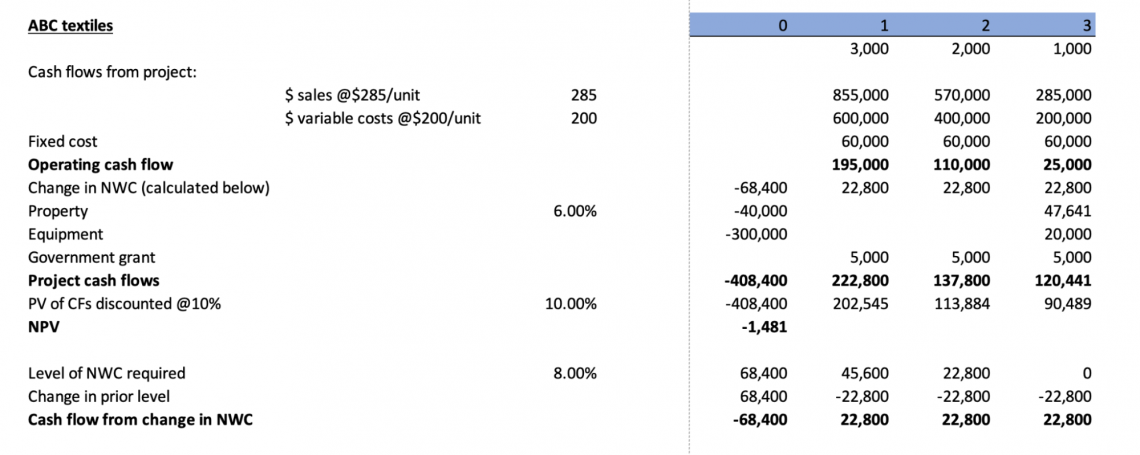
Based on a simple NPV analysis, ABC should not accept the project.
Provide a Sensitivity Analysis for the Project NPV
By creating a “What-if analysis” data table with Excel, the following sensitivity analysis for the project’s NPV based on different WACC and NWC requirement assumptions is created:
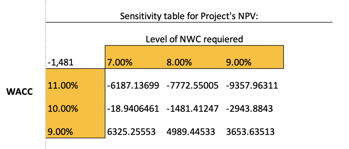
Notice how the current NPV of -1,481 becomes positive as the discount rate falls to 9%. Therefore, projects will be accepted if ABC can lower the project’s risk so that its new required rate becomes 9%.


Free Resources
To continue learning and advancing your career, check out these additional helpful WSO resources:


or Want to Sign up with your social account?