Terminal Growth Rate

In short, it is the rate at that a company is assumed to grow beyond forecasted cash flows. This is particularly important because, when performing valuation analysis, we are dealing essentially with assumptions to project our cash flows.

However, since they are all assumptions, their uncertainty rises as we go further into the periods. So we can be reasonably sure of the range of revenue growth for the next quarter, for instance, but not sure about the growth five years from now.

To account for this uncertainty beyond a certain period in our forecast, we must assume a value that represents all future cash flows beyond that particular date. To achieve that, we can either assume that the company will be sold off by a certain amount or derive a terminal value.

Since that terminal value represents the future cash flows, it is also built upon assumptions. Those assumptions, however, are different from the ones that underlie our projections. While at the start of the model, we had a lot of assumptions to build up our cash flow projections. Now we are essentially dealing with only one. 

The reason for this is that we are seeking a single amount instead of a series of cash flows. 

When we talk about cash flows, the main concern is how they will grow over time, so our main assumption will be the rate at which they will grow forever. We then use that rate to arrive at a figure that accounts for that growth into perpetuity.

That rate is exactly our terminal growth rate. 

Understanding terminal growth rate

When performing valuation analysis, we are concerned with cash flow estimates, as the company’s value is directly linked to them. However, since these future cash flows are based on assumptions, they may get a little out of touch when we stretch the projections too far into the future.

Now, let’s recap how a valuation process works. It can be done in two main ways: comparable and intrinsic valuation. The terminal growth rate is tied to the concept of cash flows, which relates to intrinsic valuation.

We use a discounted cash flow model to determine how much a business is worth in intrinsic valuation analysis. The theory behind this is that an asset is worth the future cash flows it generates discounted to the present value.

So in order to estimate these cash flows, we put in place assumptions such as revenue growth, inventory turnover rates, operating profit margins, etc. They may be accurate, but they are still assumptions. 

As we project our cash flows for future periods, we can only be so certain. There comes a time when our assumptions will hold no value due to the natural unpredictability of events.

The terminal growth rate arises from a flaw inherent to intrinsic valuations - the accuracy of the assumptions.

This is exactly where the idea of terminal value comes in. When our assumptions start to look imprecise due to being too distant, we must assume the company will generate a certain amount of cash to discount it to present value.

When faced with this issue, analysts have two choices:

1. Use the comparable companies multiples, and from then on, derive its terminal value
2. Use the growth rate using the perpetuity method.

The first method takes a comparable multiple to find what the company will be worth at a point in the future.

For example, suppose we take an EV/EBITDA multiple 8.0 times. Then, we would multiply this figure by the projected EBITDA figure and derive the enterprise value at the terminal date.

From this point onwards, both methods are the same. Once we have this value in hand, we then sum it to all the other forecasted cash flows and discount them to present value using an appropriate discount rate.

The end goal is the same. What will change between the two is how we get to the terminal value and its rationale.

In the first approach, we are using a comparable valuation technique, which may be inconsistent with the intrinsic value approach. 

For the second, which we are interested in, we assume a certain growth rate for the cash flows beyond a certain point in time, called the growth rate. 

Also, in the second method, we derive a rate at which the company will grow forever, so it is, at least in theory, based on fundamentals.

The growth rate approach is known as the perpetuity method, as it assumes the company will exist forever and grow at a constant rate.

The perpetuity method

The method is built upon Gordon’s Growth Model. It is an economic model aimed at estimating the fair value of a stock in the future, and it has two key assumptions.

• The dividends are considered cash flows
• The company will exist forever and will grow at a constant rate.

It was originally conceived to be used with dividends, but it can also be used with free cash flows as long as we assume they are the same.

It takes three inputs: the free cash flow to the firm of the last forecast, the discount rate, and the assumed growth rate.

The formula is as follows:

Terminal Value = FCFF*(1+ g)/(WACC - g)

Where g is the growth rate, we take the discount rate equal to the WACC.

Notice that the growth rate must be less than the WACC for the formula to work. The rationale behind it is that, in perpetuity, companies are not expected to grow more than their cost of capital. It just would not make sense because, in the long term, it would mean the company eventually becomes larger than the entire economy.

In simple terms, it means that a company just isn’t supposed to grow more than the risk it carries to investors.

To estimate the growth rate, we must be conservative. We can take the GDP of a particular economy as a proxy for the same.

By taking the growth rate to be lower than the GDP projections, we assume the company will not outgrow the overall economy in the long run, which would be an absurd assumption.

Once we have the terminal value figure in place, we can place it in the DCF and discount it to the present value as if it were just a regular cash flow.

Estimating the growth rate

Suppose we are conducting the valuation of Company A. With all our assumptions and calculations in place, we estimate the future cash flows for the next 5 years. Now we must estimate the terminal value.

The key question here is: How would we estimate the growth rate?

To make a sound assumption, we must keep in mind that we estimate a growth rate for perpetuity. That is, if the company were to continue growing and expanding forever, obviously, in practice, that would never be the case.

Also, remember the theory behind the estimation. We estimate the terminal value simply because we need a value to bring to the present value beyond a point our initial assumptions would no longer be reliable.

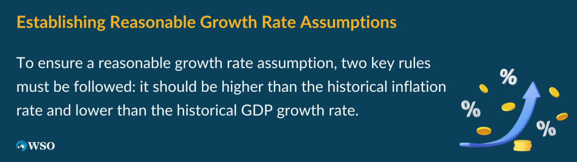
Now, to make a sanity check on our growth rate assumption, there are two key rules we must follow:

• The growth rate has to be greater than the historical inflation rate
• The growth rate has to be less than the historical GDP growth rate

To understand why our assumption must be between these two macroeconomic rates, we must first understand their meaning.

Inflation is a measure of economic activity. Since many variables get factored into the inflation figure, its headline number is not accurate for certain sectors.

When the economy heats up, prices increase, and so does inflation. So we can understand the inflation rate as a measure of economic activity.

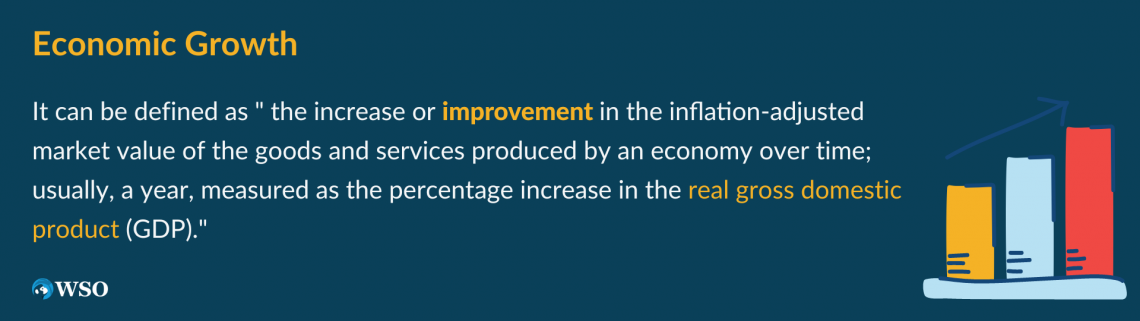
On the other hand, GDP is an indicator of economic growth and is the sum of the value-added from all the goods and services produced t in a given economy. 

We want to be conservative and thoughtful in our estimation. To achieve that, we must consider our growth rate to be higher than the historical inflation and lower than the historical GDP. 

The reason why we assume the growth rate to be greater than the inflation rate is that we are estimating the nominal figure for terminal value. So we have to consider the inflation effect.

Breaking down the calculation

The formula for terminal value takes into account three things:

1. Free Cash Flow to the Firm

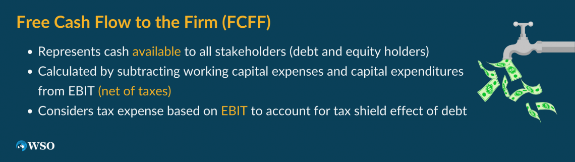
From a valuation perspective, this figure is obtained via financial modeling. It represents how much cash is available to all stakeholders (debt and equity holders) in the company irrespective of their position in the capital stack( net of taxes).

Since we want free cash flow for all stakeholders, we must subtract the working capital expenses and capital expenditures from the EBIT figure(net of taxes).

We consider the tax expense based on the EBIT figure to account for the tax shield effect of taking on debt. 

When companies take debt, they can deduce the interest expense from the tax bill. Given we are interested in accounting for all stakeholders, we must discount the tax amount from the EBIT figure. That way, we can grasp the free cash flow net of taxes.

2. Discount Rate

It is the same rate that is used in the discounted cash flow. Usually, it is the WACC. The WACC is the cost of capital for the business, and it is a weighted measure between the cost of debt and the cost of equity. We can further break it down into its two components:

1. Cost of debt: It is how much the company has to pay its debt holders to guarantee debt financing. It is the yield on the company’s outstanding debt.
2. Cost of equity: The cost of equity stands for the return investors expect to obtain from acquiring the company’s shares. It is closely related to the concept of opportunity cost, and it takes into account three distinct factors.
   1. The risk-free rate: It is the floor rate for the cost of equity calculation. Any excess return investment may yield must be above the country’s risk-free rate. Otherwise, it wouldn’t make much sense to invest in a riskier asset class without having higher returns.
   2. Equity risk premium: The equity risk premium is the extra yield compared to the risk-free rate that investors will earn by investing in the company. 

      This can be understood in terms of a risk-reward equation; if an investor is purchasing a riskier stock than others, then the reward must also be higher to compensate for the risk taken.

   3. Beta: Beta essentially measures how the company performs relative to the market. It is derived from the concept of standard deviation in statistics.

      In practice, investors use it to assess a company’s stock volatility. A beta greater than 1 means the stock is comparatively more volatile than the market, and a beta lower than 1 means the stock is more stable than the market.

      Putting it all together, we came up with the WACC, which is used as the discount rate.

3. The Growth Rate

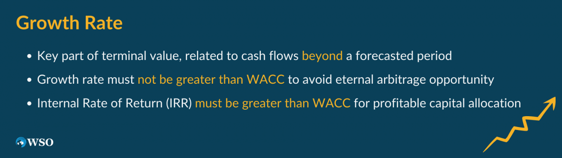
The growth rate is a key part of the terminal value as they are closely related to the same concept, the value of cash flows beyond a particular forecasted period.

Looking at the formula for terminal value, we note that the growth rate must not be greater than the WACC. But why?

Keep in mind that we are evaluating the company’s growth into perpetuity. Since the WACC is the cost of the business’s funds, if we assume the growth rate to be higher than it, we would be assuming that an eternal arbitrage opportunity would be created, which doesn’t make sense.

The internal rate of return (IRR) for the investment must be greater than the WACC for our allocation to make sense. The reason for this is rooted in the concept of risk and return. 

A company will always try to ensure that the capital is allocated to generate a higher return than the cost of capital; otherwise, it will result in an unprofitable equation for the firm.

Shortcomings

There are two main approaches to terminal value: exit multiples and the growth model.

While multiples are a relative form of valuation, in practice, they are used much more frequently because they allow a simpler and quicker calculation. Most importantly, they rely on fewer assumptions than the growth model.

Assumptions are a big element l in financial valuation and can make or break a model. The quality of assumptions relies on a fundamental feature: the timeframe for which it stands for. Short-term assumptions are much more likely to be reliable than long-term assumptions.

The shortcoming for the growth method lies exactly here, no matter how conservative our assumptions are, they are fundamentally compromised simply by being too far into the future.

Researched and authored by Lucas Amorim | LinkedIn

Free Resources

To continue learning and advancing your career, check out these additional helpful WSO resources:

• Adjusted EBITDA
• Capitalization Rate
• Sweat Equity
• Time Value of Money
• Trailing P/E Ratio