DCF Terminal Value Formula

The Terminal Value (TV) is the value of a business, project, or asset for the periods beyond the ones forecasted. It is used in determining the value of a company into perpetuity (indefinitely) beyond the forecasted periods.

When is Terminal Value (TV) Used?

The discounted cash flow model (DCF) is used by analysts when valuing a business and consists of 2 major components; the present value (PV) of its future cash flows, and its TV beyond the forecast period. The TV can be computed in 2 ways, the Gordon Growth Model and the exit multiple/terminal multiple method.

Here is a snippet from the Wall Street Oasis DCF Modelling Course to help you grasp the concepts a little better. Check out the full course here.

How to Calculate Terminal Value

TV is a major component of a DCF model and will often be the largest component of enterprise value in your model. There are 2 main ways to calculate the TV outlined below.

Gordon Growth Method

The Gordon Growth Model (GGM) assumes that a company will exist indefinitely and is consistent with the going concern assumption of financial reporting.

The growth rate for the company into perpetuity is kept constant and is usually in line with the growth rate for the overall economy as it’s mathematically impossible for companies (especially established businesses in mature industries) to grow faster than the overall economy in the long term.

The exact rate used, however, varies from company to company and industry to industry.

After a set number of years, forecasting becomes unreliable and often unrealistic, especially in high growth companies that can’t sustain such rapid growth indefinitely. To overcome this limitation, analysts assume that the cash flows grow at a specified constant rate.

The value is calculated by dividing the last cash flow by the discount rate minus the growth rate.

The Terminal Value Formula under Gordon Growth Model is:

[FCF * (1+g)]  / (r-g)

Where the variables are:

• FCF = Last forecasted cash flow
• g = terminal growth rate of a company
• r = discount rate (usually weighted average cost of capital (WACC)

Example of Gordon Growth Calculation:

FCF (at the end of Year 10) = $10,000
g = 2%
r = 6%

Based on the formula above, we can calculate the TV into perpetuity as follows:

TV = $10,000 * (1 + 2%) / (6% - 2%)
TV = $10,200 / (4%)
TV = $255,000

The terminal growth rate is the expected growth rate of the company into perpetuity and is applied to the last forecasted cash flow to provide the first cash flow past the forecasted period. 

For example, if the forecasted period ended in 2030, FCF * (1+g) would give you the FCF for 2031. The 2031 FCF is then divided by the discount rate less the terminal growth rate.

As mentioned above, the terminal growth rate should not exceed the historical growth rate of the overall economy (GDP) and should be roughly in line with inflation.

Terminal Multiple / Exit Multiple Method

The terminal multiple is another method of calculating the terminal value. This method assumes that the enterprise value of the business can be calculated at the end of the projected period by using existing multiples on comparable companies.

Commonly used terminal multiples include EV/EBIT and EV/EBITDA which can be found online or calculated from company financial statements. Another source of terminal multiples includes looking at precedent transactions.

Example of Exit Multiple Method in DCF

An EV/EBITDA multiple of 10x would imply that the enterprise value of a company is 10x its EBITDA (earnings before interest, taxes, depreciation, and amortization). For example, if a company had an EBITDA of $5,000, the enterprise value would be $50,000

The terminal multiple is applied to the final year EBITDA (or EBIT)  and is added to the cash flow of the final year. The cash flows are then all discounted at the discount rate (WACC) and gives the implied enterprise value of the business.

For companies that operate in a cyclical industry and whose performance is dependent on the business cycle, earnings will fluctuate with the overall state of the economy. For companies like this, you use the average EBIT or EBITDA over the years, rather than the final year value as this can skew your valuation.

Which Terminal Valuation Methodology is Better?

There is no one way that is better and will give you a more accurate valuation. Whichever method you choose will come down to whether you want a more optimistic or conservative estimate on TV.

Generally speaking, the Gordon Growth Model will give you a higher value while the terminal multiple method is more conservative. However, in any valuation model, using just one method can weaken your analysis.

Using both perpetuity growth and terminal multiple methods and averaging the two values is another approach to help an analyst come to a realistic valuation.

Why is the Terminal Value Important

In financial modeling and analysis, this figure encompasses the value of all future cash flows beyond the forecasted period and is based on a specific growth rate or a specific multiple.

Accurately forecasting revenue and cash flow beyond 5-10 years are difficult, and the longer out you go the more and more room there is for error, especially for something as volatile as cash flows.

As such the TV provides analysts with a simple value to add onto the PV of forecasted cash flows to determine total enterprise value from which to derive a price per share.

Limitations of Terminal Value

The TV is useful in completing a DCF model and valuing a business, however, it’s not without its shortcomings. Terminal multiples, for example, can change over time. The industry multiple this year might not be the multiple used 10 years from now. As industries mature, multiples tend to compress over the years and stabilize.

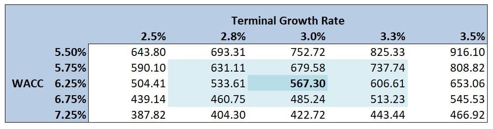
The perpetuity method brings its own set of nuances and problems. Given the nature of the formula, the TV is extremely sensitive to inputs.  For example, changing the growth rate or discount rate, even by one percent, can have a material effect on the enterprise value. 

One way of highlighting the sensitives of the perpetuity method is through a sensitivity table which shows the different values based on combinations of terminal growth rates and WACC’s.  Here is an example below of what this might look like:

Can You Have A Negative Terminal Value?

Getting a negative terminal is only possible under the Gordon Growth Model. This happens when the terminal growth rate is higher than the WACC. Intuitively this doesn’t make sense.

A company with a high growth rate should not have a negative value, right? Well, a company cannot maintain a growth level that exceeds that of the overall economy in the long term without becoming the economy. Therefore the assumption is inherently flawed and nonsensical, just like the resulting value.

Example (Remember: [FCF * (1+g)]  / (r-g))

FCF = $10,000
r = 3% (**faulty assumption** companies with the lowest WACC in the entire market are at least 4+%)
g = 5% (**faulty assumption** this implies that the business grows faster than the entire economy indefinitely which means it will, in essence, become the economy)
TV = $10,000 * (1+3%) / (3% - 5%)
TV = $10,030 / (-2%)

TV = -$51,000

So yes, if you insert absolutely moronic assumptions into the formula, you can force a negative TV. However, this is meaningless (junk in = junk out) and you should never actually encounter this in real-life valuations. 

Terminal value (TV) is the value of a business, project, or asset for periods beyond the forecasted horizon. It is primarily used in Discounted Cash Flow (DCF) modeling, where it accounts for the major part of the valuation.

When forecasting cash flows or valuing projects or companies using Discounted Cash Flow (DCF) model of valuation, the numbers are explicitly forecasted for a few years – say, 5 to 10 years.

Even though we can forecast cash flows for hundreds of years on spreadsheets with varying assumptions for each year, it tends to be quite unrealistic and imprecise over such large periods. Just because a model is extended or made more complex does not make it precise.

On the other side of the dilemma, just because we cannot reliably predict the cash flows beyond a few years does not mean that the company will not have any value at that point in the future. Hence, we still need to find the company’s value after the forecast period without explicitly modeling for each period's cash flows.

This is where we use the terminal value. It is the value of a company at that point in the future. Let’s assume that our explicit forecast horizon is 6 years. The terminal value in year 6 would be the company’s total value from the 7th year onwards.

There are many ways of calculating terminal values. The choice depends on the underlying assumptions about the company – for instance, whether the investor is seeking a conservative estimate, an optimistic estimate, or an average of the two.

Perpetuity growth method

Also known as the Gordon Growth Model, this method gives us the company’s present value at the end of the forecast horizon. This method is ideal when reasonable estimates of the future discount rate and growth rate can be made. It is used assuming that the investment has an infinite horizon as well as constant growth rates and discount rates.

Under the perpetuity growth method, the terminal value is computed as the cash flow for the next year, divided by the difference between the future discount rate and the future growth rate.

TV_t = CF_{(t + 1)} / (r – g)
or
TV_t = CF_t * (1 + g) / (r – g)

TV_t = Terminal value in year t
CF_{(t + 1)} or [CF_t x (1 + g)] = Cash flow in year (t + 1)
r = Future discount rate
g = Growth rate
r - g = Perpetual growth rate

Let’s assume that the cash flow in year t for a company is $100,000, its cost of capital (the discount rate, r) is 10%, and that the annual cash flow would perpetually grow at 2% per year (g). Using the formula listed above, the terminal value of the company in year t can be calculated as:

TV_t = [$100,000 x (1 + 2%)] / (10% - 2%)

TV_t = $1,275,000

No growth perpetuity method

This method is the same as the perpetuity growth method. However, it is used for businesses operating in industries with high competition. Thus, the growth rate for terminal value computation is assumed to be zero. It is computed as the present value of a perpetuity stream with no growth. 

Although, it may not give a good estimate of a company’s terminal value as it does not account for inflation. A business not being able to grow its cash flows at least at the rate of inflation means that it is losing money in real terms.

Assuming there is no growth in the perpetuity stream, the terminal value in year t would simply be the cash flow in year t divided by the discount rate.

TV_t= CF_(t)  / r

• TV_t = Terminal value in year t
• CF_(t) = Cash flow in year t
• r = Future discount rate

Let’s take the same example as before. We will use the same annual cash flow (CF_t = $100,000) and cost of capital (r = 10%), but this time we will assume the perpetual growth rate (g) to be zero this time.

TV_t = [$100,000 x (1 + 0%)] / (10% - 0%)

TV_t = $100,000 / 10%

TV_t = $1,000,000

Exit multiple method

The exit multiple method is ideal when investors want to assume a finite period of operations. The implicit assumption is that the investors would seek to exit the investment at the end of the forecasting horizon.

Thus, there is no need to calculate the value of a business based on perpetual cash flows. Instead, the terminal value is calculated based on financial metrics, such as:

• Earnings before interest, Tax, Depreciation, and Amortization (EBITDA)
• Sales
• Net income

Investors consider the exit multiples of other similar companies recently sold or acquired and calculate their exit multiples. These exit multiples are then applied to the forecasted financial metrics of the investment under analysis.

Multiples of publicly traded companies can be easily obtained from publicly available market data. However, obtaining data for private transactions may be easier said than done.

The exit multiples of peer companies are calculated as the recent acquisition price (market capitalization in the case of public companies) divided by a financial metric of the peer company.

Exit Multiple = Value of a peer company / Its value driver

To arrive at the company’s terminal value, we use the same financial driver as the one used to calculate the multiple and multiply it by the observed multiple.

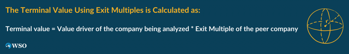
The terminal value using exit multiples is calculated as: 

Terminal value = Value driver of the company being analyzed * Exit Multiple of the peer company

Here's an example of how to calculate the terminal value using some real-life figures:

Let’s assume there is a private company ABE that is manufacturing electric vehicles and is a direct competitor to Tesla. Let’s take the PE ratio as the exit multiple. Tesla has a PE ratio of 328.47 (as of December 3rd, 2021).

We know that the net earnings for ABE in the most recent financial year have been $400 million. Applying the same PE multiple, we can determine the value of ABE to be $131.388 billion (= $400M x 328.47).

An important thing to note is that multiples can vary over time and from company to company. Continuing the same example above:

Tesla’s current PE ratio is 328.47. However, it has fluctuated between 250.88 and 1401.73 in the past year. The possible terminal values for ABE based on these two extreme PE multiples would be $100.35 billion and $560.69 billion.

That is a wide range. Therefore, to reduce the effects of such extreme cases, we can use simple averages or moving averages of exit multiples observed from a group of peer companies or industry averages. Further, we can also compute various terminal values using different value drivers and their averages.

Perpetuity Growth vs Exit Multiple methods

The two approaches have completely different starting points and are based on different rationales. Consequently, the terminal values derived from them are most likely to differ as well. But even though the approaches are vastly different, they have more in common than we might think.

When using the perpetuity growth method, a discount rate implies a certain exit multiple.

For instance, using 5% as the required rate of return and 2.5% as the rate of perpetual growth (r - g of 2.5%) implies an exit multiple of 40.

(r - g) = 2.5%

1 / (r - g) = 40

Similarly, using an exit multiple of 25 implies that the perpetual growth rate is 1% at the same required rate of return. We can relationally analyze whether these assumptions are too high or too low if we understand how exit multiples and discount rates are interlinked.

Methods of Discounted cash flow terminal value

Neither of the methods is likely to give an accurate estimate of terminal value. Choosing a method comes down to investors’ expectations. There are also some underlying assumptions and requirements that need to be met to make the best use of the different approaches.

Period of operations: Do the investors find the investment to have a finite life, or can it operate perpetually?

• If an investment has a finite life, it is best not to calculate the terminal value, but project out the DCF model over the finite period.
• Contrarily, if an investment has an infinite time horizon, it would be a good idea to account for future cash flows along with a constant growth rate.
• Furthermore, if the growth rate cannot be assumed to be constant (as is the case in startups and early-stage companies), it is best to use the multiples method.

Estimating inputs: A model is only as strong as the underlying assumptions and inputs. If the inputs cannot be estimated reliably, it leads to a classic case of “garbage-in-garbage-out.”

• To use the perpetuity growth method, we need to have a fair estimate of the future growth rate and the future discount rate with a reasonable economic rationale.
• On the other hand, to apply the exit multiple method, we need data on similar companies that were recently acquired which is good in terms of quantity and quality.
• It may not be easy to find enough recent data on other highly comparable companies. Think Apple Inc. and Microsoft Corporation. They may seem like competitors, but you will find that they have very different businesses on close inspection. An exit multiple of Microsoft may need to be greatly adjusted to be used for Apple. Moreover, data for public companies can be easily obtained from publicly available market data. However, obtaining data for private transactions may not be as easy.

Practitioners like to compare investments in relation to similar investments, so they prefer to use the exit multiple method.

Academics like the perpetuity growth method better because it is theoretically sound and has a stronger economic rationale. As both methods are interlinked, one can be used to derive the value of the other.

Regardless of the choice of approach, it is helpful to use a range of inputs for the discount rate, the growth rate, and exit multiples to have a range of valuation figures.

DCF terminal value modeling considerations

The terminal value significantly impacts the Discounted Cash Flow (DCF) analysis valuation. The following are factors to consider while calculating the terminal value while using DCF to ensure reliability in the models’ outputs.

1. The accuracy of the cash flow decreases with each year

Therefore, the accuracy of the cash flows in year n is partly dependent on the accuracy of all the cash flows from year 0 to year n.

2. Special consideration is necessary regarding uncertainty of external factors

The external factors could be economic, geopolitical, environmental, technological, legal, etc. These externalities need to be factored into the discount rate.

3. The perpetual growth rate (g) in the perpetuity growth method cannot be more than the growth rate of the country’s GDP in which it primarily operates

A growth rate of cash flows that are higher than the GDP growth rate would indicate that the company would grow faster than the economy. This cannot happen without the company becoming larger than the economy itself.

4. Exit multiples change with time and must be adjusted accordingly

Present-day multiples are different from historical multiples. Future multiples may be different from present-day multiples. Multiples may also differ from company to company. These facts indicate cross-sectional and temporal inconsistencies. Using averages is an excellent idea to lower the volatility of multiples.

5. It is crucial to consider the implied perpetual growth rate when using the exit multiple approach and vice versa

A reasonable-seeming multiple relative to the industry average may not seem as reasonable if we examine the implied discount rate.

Negative terminal value

Theoretically, it is possible to have a negative terminal value while using the perpetuity growth method. A couple of scenarios in which it is possible are given below.

► Growth rate higher than the required rate of return:

This means that the cash flows would be growing at a higher rate than the cost of capital. This is not sustainable perpetually. It is best to verify and adjust assumptions related to growth, cost of capital, or both in such a situation.

► Negative cash flows:

Terminal value should be calculated after the company has stopped making losses (as companies generally do in their early years), and when it is reasonable to assume that the operations will not need to be stopped in the foreseeable future (going concern assumption).

Calculating the terminal value with negative cash flows implies that we expect the business to lose cash forever, in which case the terminal value being negative is not wrong. This means that it might be best to employ the capital elsewhere.

Understanding these scenarios is important as arriving at a negative terminal value may not always be due to something being wrong with the model. That said, we must ensure that the assumptions behind the model are indeed rational.

In cases where the terminal value is calculated to be zero using the perpetuity growth method, it is better to use the multiples approach of calculating terminal value as this method overcomes some inherent limitations of the discounting models.

Is terminal value the same as NPV?

The terminal value is the value of an investment at the end of the explicit forecast horizon. It assumes perpetual cash inflows because we cannot reasonably predict future cash flows after a certain point.

Further, we assume a constant cost of capital (r) and growth rate for the cash flows (g), and we calculate the present value of these perpetual cash flows using the formula for perpetual growth.

Net present value (NPV) is the present value of all projected cash inflows and outflows associated with an investment. A positive NPV means that the investment will generate more money than the initial cash outlay after adjusting for the time value of money.

Free Resources

To continue learning and advancing your career, check out these additional helpful WSO resources:

• Foundations of Real Estate Financial Modeling
• How To Build A Merger Model
• Independent Variable
• Top Financial Modeling Courses
• What is Financial Modeling?